| | Conversion of soil lines from paper to ARC/INFO polygons� | Attaching attribute tables to ARC/INFO polygons
Use this link to return to the Soil Inventory Procedures Manual
The process described in Section 3.1 are for conversion of soil lines drawn on paper into ARC/INFO polygon coverage. Only the lines are converted in this process. A separate process, described in Section 3.2, connects the ARC/INFO polygons with the attribute data for the polygon information entered using the FoxPro data entry screens.�
Conversion of Soil Lines from Paper to ARC/INFO Polygons�
Step 1. Linework preparation
Linework to be converted was delivered to the Digital Data Processor on paper or mylar with:�
- At least four Alberta Township Survey (ATS) locations indicated. In most cases, the actual township outline was included on the same sheet as the linework�
- Clear, dark lines of uniform thickness�
- Lines reaching the edge of the area to be converted extending past the boundary about 0.5 cm.�
The linework could NOT have:�
- Extraneous lines other than soil lines and ATS lines�
- Polygon numbers or other annotation within the boundary of the area to be converted.�
Notes:
- Soil lines that were intended to be coincident with hydrography from the base map were NOT drawn. These lines were digitally overlaid during the conversion process.
- A photocopy of the linework (scale is not important) was provided with soil polygon numbers clearly labeling each polygon. This sheet was used in the following step.�
Step 2. Scanning�
Process� - The linework was converted to a black and white raster representation through scanning. The scanning was done using a Microtek scanner.�
Scanning was done at 200 dots per inch (dpi). This value was chosen to minimize file size and processing time while retaining all linework.�
The scan was stored as a TIFF (Tagged Interchange File Format) file.�
Output� - Raster image from scanner in TIFF format:�
Figure 3.1 Scanned soil map��
��
Step 3. Raster editing�
Input�� - Raster image from scanner in TIFF format:�
Process�� - The raster image was edited with a bitmap editor (Canvas) to remove unnecessary lines, to fill in small gaps in the image, and to ensure that the ATS corners were easily identified. In this step:�
- Unnecessary lines, especially the ATS township lines, were removed. Smudges and overlaps of lines may were also edited.�
- Gaps in the image were filled in. If the gaps were too large, the image was re-scanned after touching it up, or scanned at a higher resolution.�
- Four ATS corners were selected and the raster image edited to produce a clear reference point after conversion. The points chosen were as close to the extreme corners of the area to be converted as possible, but were separate and distinct from soil lines. The raster image of the corner appeared in the shape of a cross. The arms of the cross were uniform in width and as narrow as possible (length is unimportant). Opposite arms were required to line up exactly.�
The editing was done using Canvas. The edited file was written on the local disk as a TIFF file using 'simple compression'. Problems were encountered when using Canvas to write directly to a file on the file server.�
Once the file was written, it could be copied to the file server to be accessible for the next processing step.�
Output�� - Clean raster image, stored as a TIFF format file:�
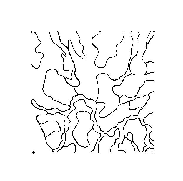
Figure 3.2 Raster edited soil map�
��
Step 4. Convert to DataPath raster format�
(The following five steps (4-8) used a software package (DataPath).�
Input�� - Clean raster image, stored as a TIFF format file:�
Process� - The TIFF raster file was converted into a format acceptable by the raster-to-vector conversion program.�
Output�� - Clean raster image, stored as a file in DataPath raster format:�
Step 5. Convert to vectors�
Input�� - Clean raster image, stored as a file in DataPath raster format.�
Process� - The raster-to-vector conversion was done on a SPARC workstation. All conversion parameters were left at the default value supplied by the conversion software.�
Output�� - DataPath format vector file in scanned raster coordinates, oriented with respect to the scanner:�
Step 6. Check and edit vectors�
Input��� - DataPath format vector file in scanned raster coordinates, oriented with respect to the scanner.��
Process� - The converted vectors were checked using the vector editor alf (on the SPARCS workstation).��
Output�� - DataPath format vector file in scanned raster coordinates, oriented with respect to the scanner.��
Step 7. Rotate and flip vector coordinates.�
Input�� - DataPath format vector file in scanned raster coordinates, oriented with respect to the scanner.��
Process� - Scans generated on the Microtek scanner were oriented with the long axis in the Y direction. Since CAESA working blocks were oriented east west, the vector coordinates were rotated through 90 degrees.��
The scanned image had its origin in the upper left corner, with X increasing to the right, and Y increasing downward. To be compatible with geographic coordinates, the Y values were converted to increase upward.��
Output�� - DataPath format vector file in raster coordinates oriented as geographic coordinates.��
Step 8. Convert to ARC/INFO format�
Input�� - DataPath format vector file in raster coordinates oriented as geographic coordinates.��
Process� - An empty file was created, and the lines in the DataPath-format file were converted into ARC/INFO 'Generate' format.��
Output�� - Linework description in ARC/INFO 'Generate' format.��
Step 9. Import into ARC/INFO�
Input�� - Linework description in ARC/INFO 'Generate' format.�
Process��� - The ARC/INFO input file prepared by dsf2arc was used to create ARC/INFO line coverage of soil lines and crosses at the corners.�
Output�� - ARC/INFO coverage of soil lines in scanner coordinates.�
� 
Figure 3.3� Soil lines after import to ARC/INFO�
Step 10. Obtain township corners�
Process� - The corners of the working area were extracted from the Alberta Township Survey (ATS) file, by specifying the township corner are to be used. The points were specified in a counter-clockwise order around the area, starting in the northeast. Whenever possible, the NE corner of a township was used as a reference.�
Output�� - File containing latitude and longitude coordinates of township corners:�
Step 11. Convert township corners to 10TM�
Input�� - File containing latitude and longitude coordinates of township corners.�
Process� - Use the USGS projection software to convert the latitude and longitude position of each corner into the provincial standard 10 degree Transverse Mercator projection (10TM), centered on 115 degrees West longitude.�
Output�� - File containing 10TM coordinates of township corners.�
Step 12. Add reference points (tics)�
Input�� - ARC/INFO coverage of soil lines in scanner coordinates.�
Process� - The linework was drawn on the screen, and a tic was added at each of the corners, centered on the crosses left from the township lines.�
Output�� - ARC/INFO coverage of soil lines in scanner coordinates, with tics located at the corners of the coverage.�
Step 13. Convert to geographic coordinates�
Input�� - ARC/INFO coverage of soil lines in scanner coordinates, with tics located at the corners of the coverage.�
File containing 10TM coordinates of tics.�
Process�� - A command file was generated, using the 10TM coordinates of the corners of the working area, which created a new ARC/INFO coverage, replaced the tics with the 10TM coordinates, and transformed the coverage.�
Output�� - ARC/INFO coverage of soil lines with coordinates in 10TM coordinates.�
Step 14. Overlay township grid and hydrography�
Input�� - ARC/INFO coverage of soil lines.�
Process� - Add township lines computed from the Alberta Township Survey, and lines representing perennial hydrography which were candidates for soil delineations.�
Output�� - ARC/INFO coverage of soil lines, township lines, and hydrography.�
Step 15. Clean up linework�
Input�� - ARC/INFO coverage of soil lines, township lines, and hydrography.��
Process� - Used the ARC/INFO editor, ARCEDIT, to be sure that the linework was reduced to polygon lines only. This step ensured that:�
- The crosses in the corners used for geo-referencing were removed�
- All lines reach the line they intersected (no 'dangles')�
- There were no gaps in the linework�
- All unnecessary hydrography lines were removed�
Output�� - Edited ARC/INFO coverage of soil lines and township lines.��
Step 16. Build polygon topology�
Input�� - Edited ARC/INFO coverage of soil lines and township lines.�
Process� - The clean linework was converted into complete polygons, with a unique (within a working area) graphical polygon number assigned to each polygon by ARC/INFO.�
Output�� - ARC/INFO coverage of soil polygons, with a graphical polygon number assigned to each polygon.�
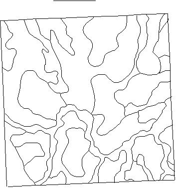
Figure 3.4 Soil lines after topology building�
Step 17. Get township attributes�
Input�� - ARC/INFO coverage of soil polygons, with a graphical polygon number assigned to each polygon.�
Process� - In order to ensure that each polygon in the entire database had a unique number, the township ID (according to the LRIS standard of Meridian Range Township, e.g., 401001) was appended to the attributes of every polygon.�
Output�� - ARC/INFO coverage of soil polygons, with a graphical polygon number and township identifier assigned to each polygon, as well as other attributes.�
Step 18. Remove unnecessary attributes�
Input�� - ARC/INFO coverage of soil polygons, with a graphical polygon number and township identifier assigned to each polygon, as well as other attributes.�
Output�� - ARC/INFO coverage of soil polygons, with a graphical polygon number and township identifier assigned to each polygon.�
Attaching Attribute Tables to ARC/INFO Polygons
This process connected the ARC/INFO polygons with the attribute data for the polygon entered into the FoxPro data entry screens. Only the attributes were attached in this process. A separate process, described Section 3.1, converted soil lines drawn on paper into ARC/INFO polygon coverage.�
1. Cross reference preparation�
A photocopy of the linework (scale is not important) was provided with soil polygon numbers clearly labeling each polygon. A plot of the linework from the previous step was generated with the graphical polygon number (GPLYNUM) from ARC/INFO displayed in each polygon.�
Notes
- it was essential that each polygon number assigned to a soil polygon be unique
- a soil polygon that crossed township boundaries within a working area had one soil polygon number assigned.
2. Load cross-reference table with graphical polygon numbers��
Process�� - Extract a file with one line for each graphical polygon number (GPLYNUM) in the Polygon Attribute table. The file was generated using INFO, then moved to a specific filename using a Unix shell command.�
3. Enter soil polygon numbers into cross-reference table��
Input�� - Paper copies of GPLYNUM plot and analyst's drawing�
Notes
- There may be several graphical polygons for each soil polygon. There was only one line in the file for each graphical polygon.
- A quick test for completeness was to compare the number of polygons reported by ARC/INFO with the number of lines in the spreadsheet. There was one more polygon than lines, since ARC/INFO counts the background polygon.�
4. Prepare temporary cross-reference table��
Process�� - Create a new INFO table, using the Cross Reference table as a template. Load the table with the values from the Excel spreadsheet.�
5. Test for typos�
Process�� - Checked to see that all graphical polygon numbers (GPLYNUM) were within the acceptable range for a work area.�
Counted the number of times each graphical polygon number occurred in the cross-reference table. If any occurred more than once, the table was corrected.�
6. Check for GPLYNUMs missing from cross-reference table.��
Process�� - Identified any graphical polygon numbers (GPLYNUM) which existed in the Polygon Attribute Table, but not in the cross-reference table. This was done by searching through the cross-reference table through a relate from the polygon attribute table. Only the ARC/INFO background polygon (always record #1) should not be found.�
7. Check for GPLYNUM entries not in polygon attribute table.�
Process�� - Identified any graphical polygon numbers (GPLYNUM) which existed in the cross-reference table, but not in the Polygon Attribute Table. This was done by searching through the Polygon Attribute Table through a relate from the cross-reference table. No polygons should have been found. Any that were found likely represented polygons that were deleted from the ARC/INFO coverage, and were deleted from the cross-reference table.
8. Prepare plot of soil polygons smaller than guideline.�
Process�� - Prepare a plot which highlighted soil polygons smaller than 65 ha. This was done by using the area stored in the polygon attribute table.�
Output�� - Plot highlighting polygons with areas smaller than 65 ha .�
9. Check for soil polygon continuity.��
Process�� - Highlighted lines that have identical soil polygons on either side. This should result in the interior township lines of the working area. Gaps in these lines indicate that soil polygons are broken across township lines. Other non-township lines indicate duplicate soil polygons. In either case, the soil polygon numbers on either side of the lines were checked.�
Output�� - Plot of lines with identical soil polygon numbers on both sides.�
10. Import data tables��
Process�� - Data was loaded into info tables that were structured to match the FoxPro tables. The first step was to remove the quotation marks from the FoxPro export files. The delimiter character used was a TAB, since commas appeared in the slope field. The number of records imported was compared to the number of records exported from FoxPro to be sure no records were lost.�
11. Add items to data tables.�
Process�� - An item (SOILPOLY) was used in both attribute data tables to link to the cross-reference table. The value of this item was calculated from the legal description fields.�
12. Check for polygons in the attribute tables that are not in the cross-reference table.�
Process�� - Identified any soil polygons (SOILPOLY) which existed in the attribute tables, but not in the cross-reference table. This was done by searching through the cross-reference table through a relate from one of the attribute tables for legitimate GPLYNUMs. All other soil polygons were not in the cross-reference table. No polygons should be found. Any that are found likely represented polygons that were missing from the ARC/INFO coverage.�
Also checked to see that there was meaningful data in the MAS table, by checking that the mandatory field MAS_EXT (extent) was not blank.�
13. Check for polygons missing from the attribute tables.�
Process�� - Identified any graphical polygon numbers (GPLYNUM) which existed in the Polygon Attribute Table, but not in the attribute tables. This was done by searching through one of the attribute tables through a relate from the polygon attribute table. Only the ARC/INFO background polygon (always record #1) was not found.�
14. Build temporary evidence table.�
Process�� - Build a new table (EVDDBF), with an identical structure to MASDBF, which contained both evidence entered in the MASDBF table by the analyst, as well as evidence filled in by looking up the symbol and variant in the soil names file (SNFDBF).�
15. Generate preliminary soil landscape models.�
Process�� - Apply the rules for soil landscape model generation to the evidence in the temporary evidence table, and stored the preliminary symbol in the SLADBF table.�
16. Highlight lines, which have identical soil landscape models on both sides.�
Process�� - Selected lines from the graphical coverage that had identical soil landscape models on both sides. The resulting lines should be the interior township grid for the area. Gaps in this grid indicated soil polygons split across the township line. Additional lines indicated possible redundancy in the mapping process. The analyst checked the soil data in the polygons on either side of the line to see if the line should be removed, and the two polygons united.�
Output�� - Plot�
Rules for Soil Model Number Generation
The soil model number indicates the presence of a soil characteristic that is not part of the soils in the dominant or co-dominant part of the soil symbol.�
The process used to determine the soil model number translates the measure of each soil characteristic to a severity category. One category is computed for the dominant soils (those mentioned in the soil symbol - D or C1 and C2), and a second category is computed for the significant soils. In the case of multiple dominant or significant soils, only the extreme (maximum or minimum) measure is recorded. The extreme measures of each characteristic are compared, and any that are more extreme in the significant soils than the dominant soils are included in the computation of the soil model number.�
For example, given the following soils:�
| Name� | Extent | Wetness | Parent Material |
| WLN� | C1 | FD | M3 |
| LTZ� | C2 | I | C2 |
| AGC� | C3 | FD | F1 |
| MDF� | S1 | P | C3 |
The categories for each characteristic would be assigned:
| Name� | Extent | Wetness | Parent Material |
| WLN� | C1 | 1 | 2 |
| LTZ� | C2 | 2 | 3 |
| AGC� | C3 | 1 | 1 |
| MDF� | S1 | 3 | 3 |
The extreme category of each of three characteristics (drainage-2, fineness-5, and coarseness-6) would be evaluated as:
| Soil� | 2 Wetness
(Maximum) | 5 Fineness
(Minimum) | 6 Coarseness
(Maximum) |
| Dominant� | 2 | 2 | 3 |
| Significant� | 3 | 1 | 3 |
So the individual numbers would be 2 and 5, which is represented by a soil model number of 18.�
�
Soil Model Number Generation process
Step 1. Calculate individual numbers
- For each soil, assign a category representing each characteristic.
- For each polygon, calculate two extreme categories, one for dominant soils, and one for significant soils.
- For each polygon, compare the extreme significant category and the extreme dominant category, to calculate all individual model numbers which apply.�
Number | Characteristic to be represented | Computation | Comparison |
2 | Wetness | Maximum Wetness Category | Sig > Dom |
3 | Salt-affected | = 1 if symbol = 'ZNA' or
modifier contains 'SA' or
variant contains 'SA'
= 0 otherwise | Sig > Dom |
4 | Regosolic | Ignored if landscape modifier is 'e'
= 1 if order = 'REGO' or
(subgroup is 'R.*' and order is not 'GLEY')
or
variant is 'ZR','ER',or 'CR' or
symbol = 'ZER'
= 0 otherwise | Sig > Dom |
5 | Fineness | Minimum Parent Material Category | Sig < Dom |
6 | Coarseness | Maximum Parent Material Category | Sig > Dom |
7 | Solonetzic | = 1 if order = 'SOLO' or
symbol = 'ZSZ'
= 0 otherwise | Sig > Dom |
16 | Chernozemic | = 1 if order = 'CHER' or
subgroup = ‘D.GL’ or ‘GLD.GL’
= 0 otherwise | Sig > Dom |
20 | Dryness | Minimum Wetness Category | Sig < Dom |
21 | Organic | Sig = 1 if order = 'ORGA', = 0 otherwise.
Dom = -1 if order = 'ORGA',
Dom = 1 if order = 'GLEY' and no 'ORGA',
Dom = 0 otherwise. | �
Sig = 1 AND
Dom = 1 |
Step 2. Compute the soil model number��
For each soil polygon, find the first number which matches the candidate numbers, following the order in the table below:
| � | Individual number |
Composite (final)Number | 2 | 3 | 4 | 5 | 6 | 7 | 16 | 20 | 21 |
19 | X | � | � | � | � | � | X | � | � |
18 | X | � | � | X | � | � | � | � | � |
17 | � | � | � | X | � | X | � | � | � |
15 | � | � | � | � | X | X | � | � | � |
14 | � | � | X | � | � | X | � | � | � |
13 | � | X | X | � | � | � | � | � | � |
12 | X | � | X | � | X | � | � | � | � |
11 | � | � | X | � | X | � | � | � | � |
10 | X | � | � | � | � | X | � | � | � |
9 | X | � | � | � | X | � | � | � | � |
8 | X | � | X | � | � | � | � | � | � |
21 | � | � | � | � | � | � | � | � | X |
7 | � | � | � | � | � | X | � | � | � |
3 | � | X | � | � | � | � | � | � | � |
6 | � | � | � | � | X | � | � | � | � |
5 | � | � | � | X | � | � | � | � | � |
20 | � | � | � | � | � | � | � | X | � |
16 | � | � | � | � | � | � | X | � | � |
4 | � | � | X | � | � | � | � | � | � |
2 | X | � | � | � | � | � | � | � | � |
�
Polygons which do not have a number assigned are considered to be homogeneous, and are assigned soil model number 1.�
��
Severity category tables:�
2: Soil wetness
Category | MAS_WET |
1 | FD, I |
3 | P |
4 | AP |
5 and 6: Texture
Category | Parent Material (MAS_PM) |
0 (ignored) | P1, P2, P3, U0, missing� |
1 | F*, L6, L13, L14, L15, L16� |
2 | L3, L8, L10, M0, M1, M2, M3, M4, M5� |
3 | C0, C2, C3, C4, C5, C6, C7,�L1, L2, L4, L5, L7, L9,�L11, L12, L17, L18, L19, M6� |
4 | C1� |
MAS_PM | PARENT | MAS_PM | PARENT | MAS_PM | PARENT |
missing | 0 | L1 | 3 | M0 | 2 |
C0 | 3 | L2 | 3 | M1 | 2 |
C1 | 4 | L3 | 2 | M2 | 2 |
C2 | 3 | L4 | 3 | M3 | 2 |
C3 | 3 | L5 | 3 | M4 | 2 |
C4 | 3 | L6 | 1 | M5 | 2 |
C5 | 3 | L7 | 3 | M6 | 3 |
C6 | 3 | L8 | 2 | P1 | 0 |
C7 | 3 | L9 | 3 | P2 | 0 |
F0 | 1 | L10 | 2 | P3 | 0 |
F1 | 1 | L11 | 3 | U0 | 0 |
F2 | 1 | L12 | 3 | � | � |
F3 | 1 | L13 | 3 | � | � |
F4 | 1 | L14 | 1 | � | � |
F5 | 1 | L15 | 1 | � | � |
F6 | 1 | L16 | 1 | � | � |
| � | � | L17 | 3 | � | � |
| � | � | L18 | 3 | � | � |
| � | � | L19 | 3 | � | � |
|
|