| | Ecological stratification of Alberta | Land system inventory | Soil landscape inventory | Field inspections | Correlation
Use this link to return to the CAESA: Soil Inventory Procedures Manual
The soil inventory process can be generalized into three broad functions:
a)� Compiling existing resource information or developing new resource information;
b)� Mapping and coding the soil and land attributes; and
c)� Developing information products (reports and maps).
The process is often iterative, and different functions may be done concurrently. The process is also hierarchical, that is, large tracts of land are subdivided into smaller pieces at each scale of inventory (Figure 1.2).
�
Ecological Stratification of Alberta
The CAESA Soil Inventory Project adopted principles of ecological land classification as a basis for soil inventory. Hierarchical subdivision of the earth's surface into areas of similar biological and physical characteristics is the basis for ecological stratification. Ecological units combine the characteristics of climate, physiography, soils, and vegetation into single cartographic areas (Strong and Anderson 1980). Uniformity and specificity of the area descriptions is scale dependent (larger the scale, more detail).
Ecological land classification is a hierarchical system. There are various identified levels of generalization, which comprise the classification system. The terminology used to describe the different hierarchical levels has changed with time. The different terms used to describe the similar levels of generalization within the system are illustrated (Table 2.1). Even though different names were used for labeling the different hierarchical levels, the general concepts have remained constant. The highlighted terms in Table 2.1 are the proposed standard terminology of the Ecological Land Classification System (Ecological Stratification Working Group 1995). The terminology and associated descriptions were based on the Ecoregions Map of Canada developed by the Environment Canada, State of the Environment Reporting (SOER) and Agriculture Canada, Center of Land and Biological Resources Research (CLBRR) Ecological Stratification Working Group (1995).
Soil analysts used an ecological hierarchy as an integral component in the preparation of the soil landscape database. The initial step involved the subdivision of the study area using the national ecological land classification framework. The first steps of the top down mapping approach were based on nationally correlated ecological maps to the Land Resource Area level of generalization. This framework provided a context for subsequent stratification of Land Systems and Soil Landscapes for this project.
�
Ecozone
The ecozone is an area of the earth's surface, representative of large and very generalized ecological units characterized by interactive and adjusting abiotic and biotic factors (Wiken 1986). Generally ecozones are depicted at scales <1:10M and have delineations generally ranging from 15M-150M hectares. A combination of physiographic provinces (Bostock 1964) and ecoclimatic provinces (Ecoregions Working Group 1989) define the ecozones. Five ecozones were recognized within Alberta (Wiken 1986), namely:
Prairie (Plains)
Boreal Plains
Taiga Plains (restricted to outliers)
Taiga Shield
Montane Cordilleran
A typical description of an Ecozone is: "The Prairie Ecoprovince (Ecozone) is characterized by a severe mid to late summer drought caused by low precipitation and high evapotranspiration. It is dominated by herbaceous vegetation capable of withstanding a drought, and Chernozemic soils" (p.10 Strong and Anderson 1980).
�
Ecoregion
An ecoregion is part of an ecozone characterized by distinctive ecological responses to climate as expressed by the development of vegetation, soil, water, fauna, etc. (Wiken 1986). Ecoregions are depicted at scales of 1:1M - 1:7.5M. Within the Canadian context, delineations range from 1.5M-12M hectares. Ecoregion maps for Alberta (Figure 2.2) are depicted at scales ranging from 1:1M - 1:5M.
There are 17 ecoregions recognized in Alberta (Ecological Stratification Working Group 1995). These regions were defined on the basis of ecoclimatic regions (Ecoregions Working Group 1989), physiographic subdivisions (Bostock 1964) and ecoregions and ecodistricts (Strong 1992). For provincial scale representation, the 17 ecoregions were further subdivided into 46 sub-regions based on detailed climatic, physiographic and soil development data.
An example of a sub-ecoregion is the Cooking Lake moraine, east of Edmonton. This area was too small to depict on the national scale ecoregion map. However, on the provincial scale it is recognized as a Low Boreal sub-region within the Grassland transition / Alberta Plain ecoregion.
�
Ecodistrict (LRA)
An ecodistrict is defined as part of an ecoregion characterized by distinctive assemblages of relief, geology, landforms, soils, vegetation, water and fauna (Wiken 1986). In Alberta, the Ecological Working Group (Ecological Stratification Working Group 1995) subdivided the 17 Ecoregions (and the 46 sub-regions) into 136 Ecodistricts, with a minimum size of approximately 10 townships (93,000 ha). Ecodistricts are depicted at a map scale of 1:1M - 1:2M. Within the national context, delineations generally range from 100 000 - 500 000 hectares.
The Ecodistrict map (Section 4, Figure 4.1) represents a revision and an extension of the earlier Agroecological Resource Areas (ARA) map that only covered the White Area of the province. The Ecodistrict map recognizes ecological units across the province. Also, national ecoregion and provincial Soil Correlation Area concepts were incorporated in the delineation of ecodistrict units.
Ecodistricts are described in terms of climate; predominant soils to Great Group level; predominant texture of the materials; and predominant landform. These attributes are identical to those used previously to describe ARAs (Pettapiece 1989). For example, the description for the Cooking Lake ecodistrict includes: the Low Boreal sub-ecoregion of the Grassland transition / Alberta Plain ecoregion; 3H climate; Gray Luvisolic and Dark Gray soils; loam to clay loam materials and hummocky landforms.
In order for the ecodistrict map to be as useful as possible, the ecodistrict units must be easily identifiable and reflect land use. Regional climate (as generally expressed by vegetation) is used as the first consideration for delineation of ecodistricts. Climate is usually difficult to delineate but changes in climate nearly always coincide with major physiographic breaks. Consequently, more stable and identifiable physical features are used whenever possible to define map delineations. Delineations at the ecodistrict level with minor adjustments to the ecoregion boundaries reflect local material, landforms and soils.
Boundary decisions are also aided by considerations of minimum size and land use. For example, sandy parent material in the Wainwright area was seen to have more significance for agriculture than the definition of the Dark Brown - Black soil zone boundary. Consequently, the ecodistrict boundary was adjusted to reflect the sandy soils.
In Alberta, the Ecoregion and Land Resource Area maps define the higher level strata for the present CAESA Soil Inventory Project (SIP). The CAESA SIP mandate was to compile information on the next two layers of the hierarchy, namely Land Systems (1:250 000) and Soil Landscapes (1:100 000). Application of this soil mapping approach, based on hierarchical ecological concepts assisted in the development of consistent and standardized provincial soil map products.
Figure 2.1 Ecoregion Map of Alberta (Pettapiece pers. comm. 1993).
Table 2.1 Correlation of Ecological Terms Used in Canada Since 1969.
Lacate (1969)
� | Strong (1980) | Wiken (1986) | Kocaoglu (1990)� | SOER/CLBRR�
Ecological�
Working Group
(1993) |
| � | Ecoprovince� | Ecozone
�
�
Ecoprovince
� | � |
�
�
Ecozone
�
�
� |
�
�
�
�
�
�
�
�
Land Region
1:1-3M |
�
�
�
�
�
�
�
�
Ecoregion
1:1-3M� |
�
�
�
�
�
�
�
�
Ecoregion
1:1-3M | Region
1:3M or greater
�
�
�
�
Section
1:1-3M | Ecoregion
1:7.5M�
National� |
Land District
1:500K-1M | Ecodistrict | Ecodistrict | District
1:500K-1M | Ecodistrict
Land Resource Area�
�
�
1:1M-1:2M� |
Land System
1:125-250K |
Ecosection |
Ecosection |
Geomorphic�
System
1:50-250K |
Land System
1:250K-1M� |
| � |
Ecosite | � |
Geomorphic�
Unit | � |
Land System Inventory
A Land System is a subdivision of an ecodistrict and is a real segment of the earth's surface. Land Systems within one ecodistrict are recognized and separated by differences in one or more of: general pattern of land surface form, surficial geological materials, amount of lakes or wetlands, or general soil pattern. All Land Systems within one ecodistrict have the same general climate for agriculture but differences in microclimate patterns can be recognized. An average-sized Land System is approximately three to four townships (32,000 hectares); the minimum sized Land System is approximately 1 township (9325 hectares) (Figure 2.2).
Some previous soil survey projects have described similar entities variously called Land Units (Pettapiece 1971; Kocaoglu 1975), Soil Groups (MacMillan 1987) and more recently, Land Systems (MacMillan, Nikiforuk and Rodvang 1988; Brierley, Andriashek and Nikiforuk 1993). Most other soil survey reports presented information on the regional distribution of the various attributes used to define Land Systems (landform, physiography, geology, climate, vegetation, generalized soils), but did not collate this information to delineate and describe Land Systems.
�
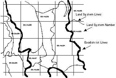
Figure 2.2 Sample Block Of 16 Townships At 1:250 000 Scale Illustrating Typical Size Of Land Systems.
�
Reasons for doing 1:250 000 land system inventory
The reasons for conducting Land System Inventory included:
1.� It is a useful and necessary step in the process of soil inventory by a top-down mapping approach.
2.� Land Systems are used for municipal - level soil and water conservation planning and program delivery. Many users (researchers, agriculture fieldmen, assessors, range ecologists) stated that Land Systems are important.
3.� The Land Systems Inventory will be used by Agriculture Canada as a basis to modify the general Soil Landscapes of Canada - Alberta map (Agriculture Canada 1988).
Land system inventory process
The recognition and delineation of Land Systems was based on integration and interpretation of a variety of data sources. Type, texture and surface form of geological deposits were used as primary criteria in subdividing ecodistricts into Land Systems. The preferred source documents to guide this subdivision were the maps of Quaternary Geology of Southern and Central Alberta (Shetsen 1987, 1990). These were supplemented with aerial or satellite imagery, local maps of surficial geology, and existing soil maps.
Subdivision of ecodistricts into Land Systems was also influenced by differences in bedrock geology, hydrogeology and surface drainage pattern. The relative hardness or softness of underlying bedrock often affects the development of drainage systems and is reflected in the degree of integration or disruption of drainage and the depth of incision of streams or rivers. The primary source document (used to guide the subdivision of map areas according to bedrock geology) was the Geological Map of Alberta (Green 1972). Large scale topographic maps provided additional guidance, especially if bedrock geology was reflected by patterns of topography or drainage.
Natural vegetation or imposed land use, as revealed on photos and satellite imagery, provided useful clues to such attributes as depth to bedrock, degree of salinity, wetness and depth to water table. Major differences in natural vegetation or imposed land use were used to guide the subdivision of ecodistricts into Land Systems. These differences were revealed by examination of aerial photos and satellite imagery.
The process of locating Land System boundaries requires understanding of what a boundary condition might be. The list of recognized Land System boundary conditions is as follows:
1.� An ecodistrict boundary
(that may be:)
- an ecoregion boundary.
- an "inferred agro-climate change boundary" based on elevation, or cropping pattern, or other evidence.
- a bedrock-type boundary.
- a change in regional surface form (e.g. from hilly upland to plain).
- a change in regional surficial geology (e.g. from moraine to dune field).
- a change in the density/size of lakes and wetlands.
- a change in regional Soil Assemblages.
and, within ecodistricts
2.� A change in regional surface forms (usually a change in pattern of forms) such as hummocky versus ridged.
3.� A change in regional surficial geology (usually a change in the assemblage of materials) e.g. glaciofluvial to eolian.
4.� A change in density or size of lakes and wetlands or a Land System may be a lake or a large wetland.
5.� A change in regional Soil Models (for example a change in dominance of Solonetzic or Gleysolic or Luvisolic).
The recommended procedure for placing Land System boundaries (i.e. mapping) and for coding attributes is described in the Land System Inventory Process and in Section 4.1 (Land System data capture). This procedure involves two groups of functions:
1.� Recognizing and checking the ecodistrict boundaries, and
2.� Subdividing the ecodistrict into Land Systems.
Steps in the land system process
Soil analysts were encouraged to use the following steps for delineating Land Systems:
1.� Obtain base maps at 1:250 000 scale. These maps included:
- township grid and hydrography (derived from the 1:20 000 provincial base) on mylar
- contours (from the 1:20 000 provincial base) on paper or mylar
- outline of block on mylar.
2.� Gather information. The information included resource maps, reports, point data. Scales were adjusted as required for overlays.
3.� Obtain the conversion database of soil names for the area
4.� Obtain existing Land Systems maps (from existing soil survey reports or conservation plans) for the area and incorporate the information.
5.� Overlay LRA lines on satellite imagery. Reconcile to SCA lines if necessary and move the lines if necessary at the 1:250 000 scale. Reconcile ecodistrict lines to agricultural land use (usually forage vs. annuals)
6.� Obtain bedrock boundaries from Green (1972) and place on an overlay of satellite imagery, contours and hydrography.
7.� Identify surficial geology patterns from Shetsen (1987; 1990) and place on overlay of satellite imagery, contours and hydrography.
8.� Identify regional soil patterns from soil maps (changes in soil zones or materials, Chernozemic vs. Solonetzic, Chernozemic vs. Luvisolic, large wetland areas) and reconcile to surficial geology, bedrock geology and land use patterns if possible.
9.� Identify surface form patterns from Shetsen (1987; 1990), soil maps and contours (1:50 000 contours reduced to 1:250 000 work better than 1:250 000 contours) and reconcile to 3, 4, 5 & 6 (above).
10.� Confirm agroclimate characteristics, changes and classification across the area. Data sources to check are ecodistricts, SCAs - soil zones, Land Capability for Arable Agriculture in Alberta climate map and cropping patterns.
11.� Produce Land Systems (by a combination of subdivision or aggregation of areas) with recurring combinations of agricultural land use, bedrock type, surficial geology, regional soils, surface form, and agroclimate. The mean size of a land system is 3 to 5 townships; minimum size is approximately one township.
12.� Code the attributes as defined by the Land System data form (Appendix A).
13.� Edge-match to adjacent blocks.
Soil Landscape Inventory
A Soil Landscape is a segment of the earth's surface with specific geographic location and extent. It is a subdivision of a Land System. Soil Landscapes within a Land System were recognized and separated by differences in one or more of: land surface form; surficial geological material(s); soil patterns (including amount of lakes, wetlands and wet soils). An average sized Soil Landscape is approximately 500 - 1000 hectares (2 to 4 sections); minimum size is 65 hectares (1/4 section).
Soil Landscapes are areas of land which display a consistent and recognizable pattern of distribution of soils and landscape elements. Most historical and recent soil mapping in Alberta focused on describing and delineating Soil Landscapes. The CAESA Soil Inventory Project benefits from and uses existing maps in which Soil Landscapes have been delineated at various scales (1:30 000 to 1:190 000). Soil analysts had two primary activities in the project. The first was to use existing maps and data to apply a uniform and consistent set of Landscape models to the entire White Area. The second was to capture and record basic soils evidence, so that an automated set of rules could be run to generate a Soil Landscape Model symbol for each delineated polygon.
�
Soil landscape inventory process
A 9 stage process was used for soil map compilation.
Stage 1 - background data
- The Digital Data Processor (DDP) provided the soil analyst a hard copy of the ATS (Alberta Township Survey) township grid and the 1:20K contours and hydrography for a Working Area. The Working Area (WA) was on average 3 ranges wide by 2 townships high (working areas varied in size).
- In addition the analyst obtained additional background information. The information included:
- Base information plotted on acetate (1:20 000 contour lines and hydrography)
- ATS grid for working areas (1 copy plotted on acetate)
- Preliminary Land System maps and descriptions for the area
- Existing soil maps (scaled to 1:100 000)
- Point data (pipeline reports, irrigation land classification, environmentally significant areas reports, public land
reports, Alberta Soil Survey Township Plans, rural assessment sheets)
- Surficial and bedrock geology maps and reports
- Topography maps (1:50 000, 1:20 000)
- Aerial photographs
- Satellite imagery (1:250 000)
- Soil names file (SNF)
- Soil layer file (SLF)
- Soil series descriptions
Stage 2 - working draft maps and data
- The analyst compiled the soils information for each Working Area, reviewed the information with the Block Leader and delivered soil lines (hand drawn, hard copy) and attribute data (digital copy) to the DDP. Analysts were encouraged to use the following process for soil map compilation:
1.� Review land system attributes. Identify attributes of Land Systems that were relevant to the soil landscape mapping being conducted. The Land Systems map that the analyst used was a draft copy. Some concepts, lines and numbers were in the Land Systems map changed during the course of Soil Landscape mapping
2.� Review soil landscapes mapped in adjacent townships to identify edge matching requirements.
3.� Compile soil lines. Soil map compilation varied depending upon the scale of the existing information. For 1:50 000 maps, the process for delineating soil landscapes was to generalize existing lines. The analyst traced lines from the 1:50 000 maps and combined polygons that were smaller than minimum size (65 ha) with larger polygons. For 1:126 000 maps, the process for delineating soil landscapes was to either use existing lines as is or the analyst revised lines based upon photo interpretation of landscapes. If the analyst desired, he or she consulted other data sources to modify soil lines and increase the reliability of the soil mapping. For 1:190 000 maps, the process for delineating soil landscapes was to use aerial photography and other sources of information to derive a new set of polygons compiled at 1:100 000 scale. The analyst used existing 1:190 000 soil maps as background information only.
4.� Code soil landscape attributes for each delineation. Coding of soil landscape attributes occurred as the soil polygons were compiled. Analysts recorded the evidence known about the polygon. Analysts did not provide interpretive information. The attributes that were required to be coded included:
- Polygon identification (meridian, range, township and polygon number)
- Land system number
- Date compiled and analyst name
- Soil model attributes
- Wetness
- Order, Great Group, Sub-Group, Soil Series (one of these)
- Parent material
- Extent
- Landscape model (or surface form, relief and slope)
- Salt affected
- Old soil map label
- Sources and source ID
- Confidence level
- Field check required
5.� Field check soil landscape boundaries and attributes. The level of effort was adjusted to account for availability and quality of resource information. The level of effort varied depending upon the scale of existing mapping. There was no field checking of 1:50 000 soil maps. The rates of field checking for areas compiled using 1:126 000 soil maps was limited to 1/4 day per township. The rates of field checking for areas compiled using 1:190 000 soil maps was limited to 1/2 day per township. These rates were guidelines for field checking. Analysts were recommended to visit specific problem areas within mapping blocks and not necessarily visit every township.
6.� Correlate. The analyst and the block leader reviewed the working area to ensure that the attributes required for each polygon were entered and that the guidelines for soil mapping listed in Section 2.3.4 were met.
7.� Revise coded attributes. As necessary upon completion of Step 3.
Stage 3 - first draft hard copy and data
- The DDP entered the data compiled for each Working Area (the process as defined in section 3.1 of this manual).
- After entering the data, the DDP ran queries on the polygons to find errors, anomalies and omissions. The DDP provided the analyst back 4 hard copy maps; a soil map with generated map symbols plotted; a plot showing polygons that were smaller than minimum size; a plot highlighting polygons that were missing basic evidence; and a plot of the soil lines highlighting lines that separated areas with identical map symbols. The DDP also provided the analyst the attribute data (digital copy) for additions or deletion of polygons.
Stage 4 - second draft hard copy and data
- The analyst made the required corrections and returned the corrected digital file (attributes) and corrected hard copy map (lines) to the DDP. The analyst corrected only those polygons that were identified as having problems in Stage 3.
- The analyst provided a list of the polygons that were changed in the database to the DDP. These were the only polygons that the DDP updated in the database. Failure to provide this list meant that the changes were not incorporated into the final database.
Stage 5 - second draft of digital data
- The DDP made the necessary corrections to the soil lines in each Working Area.
- The DDP joined the working areas into a Correlation Block (CB) (an area about 20 to 36 twp)
- The DDP forwarded the digital files (lines and attribute data) for a completed Correlation Block to the Block Leader.
Stage 6 - correlation using ArcView
- Block Leaders were responsible for ensuring continuity of lines and concepts between the working areas (see section 2.5, for a detailed description of the Block Leader roles and responsibilities).
- The Block Leader reviewed the soil maps and attributes for a Correlation Block (using ArcView) and made changes to the soil maps. The changes to soil lines were forwarded to the DDP for update.
- The Block Leader made changes to the attribute data in FoxPro and forwarded the changes for the Correlation Block (on disk) to the DDP.
- The Block Leader entered additional soil polygons using FoxPro.
Stage 7 - interim final product
- The DDP made the required changes to the soil lines and attribute data. The required changes included all edge matching of lines between Working Areas and Correlation Blocks.
The Project Leader then delivered the completed Correlation Block to the Technical Authority.
Stage 8 - Agriculture and Agri-Food Canada review
- Areas were reviewed by the Agriculture and Agri-Food Canada correlators on an SCA by SCA basis. Changes to the data were forwarded to the Project Leader for incorporation into the final database.
Stage 9 - incorporation of the correlation changes
- Changes suggested by the Agriculture and Agri-Food Canada correlators were incorporated into the final database by the Project Leader.
Soil landscape models
The Soil Landscape Model is a conceptual entity that presents a summary of the principal characteristics of several areas of land that are more or less similar. The Soil Landscape Model describes a repeating pattern of soils and landscapes that can be identified on aerial photographs and in the field by an experienced soil mapper. Soil Landscape Models:
1.� Permit a soil mapper to describe a particular combination of soils and landscapes and apply that description to areas having similar combinations of soils and landscapes
2.� Help the mapper summarize concepts about where and how soils are distributed in the landscape. This information is important to some users of the information.
3.� Provide the Block Leader a useful correlation tool and help in maintaining consistency between analysts.
4.� Provide some users a convenient basis for interpreting combinations of soils and landscapes.
A Soil Landscape Model may be thought of as an amalgamation of two models as illustrated in Figure 2.4. The basic building blocks are the Soil Model and the Landscape Model. The Soil Model is a composite of the dominant, co-dominant and significant soil series. The Landscape Model is a composite of the morphology, genesis, relief, slope class and surface form modifier attributes.
Defining a soil landscape model
The following rules apply to the definition of a Soil Landscape Model:
1.� The landscape model that most accurately describes a landscape, was selected from Table 4.11 (Section 4.0). If no existing Landscape models accurately described an area, a new Landscape model was defined based on the characteristics of the area in question. The newly defined (described) model required approval of the correlation team before it was added to the data dictionary. The Landscape model consists of morphology, genesis, modifier, relief and slope modifiers. Slope class gradients that most accurately describe the dominant slope class in the landscape were identified.
2.� The dominant soil or soils that occur within the landscape of interest were identified by series name. The primary considerations were parent material texture and dominant soil classification.
3.� A Soil Model number identified the minor (significant) soils that occurred within the landscape of interest. The primary intent was to recognize the presence of significant (� 10 - � 30%) soils.
4.� An automated set of rules was applied to the evidence collected to generate the Soil Landscape Model.
Guidelines for soil landscape mapping
The following guidelines were used for the delineation of soil landscapes:
- the Soil Landscape map should average 10 to 20 delineations per township (excluding water bodies) (approximately 500 - 1000 ha per delineation).
- minimum sized soil delineations (65 ha) met at least one of the strongly contrasting criteria, that is:
�
- the surface form is sufficiently contrasting that the landscape model changes
- the parent material is sufficiently contrasting that there is a change of at least one texture group, with the
classes being: 1) Very Coarse, 2) Moderately Coarse, 3) Medium, 4) Fine and Very Fine, and 5) Organic.
- the soils are sufficiently contrasting that there is a change in the dominant or codominant soil used as basic evidence. This usually means a change in Soil Order (Chernozemic to Solonetzic or Luvisolic to Gleysolic, etc.).
- delineated stream channels and valleys should be more than 300 m wide, and 6 km long (i.e. polygons should be at least 3 mm wide and 6 cm long at 1:100 000 scale).
- Water bodies (> 65 ha) were captured and automatically drawn from the base map hydrography. That is, the soil analyst was not required to trace the water body boundary. Rather the analysts tied their lines to the lake boundary. The analyst also entered the basic evidence for the water body.
�
�
�
Figure 2.3� Components of a Soil Landscape Model
�
Guidelines for soil landscape map coding
The following guidelines were used for the coding of the attributes of soil landscapes:
- The analyst entered the basic evidence for a polygon.
- The analyst had the option of importing evidence from an existing polygon.
- If an analyst was working in an SCA transition zone, the analyst chose the SCA which best described
the polygon.
- The order of coding basic evidence was important because the order that soils were coded was used to generate the Soil Model.
Conventions for creating symbols for soil landscape models
The following guidelines were based upon recognizing proportions of soils and associated modifiers as basic evidence for each polygon. The Landscape Model symbol obtained from Table 4.11, was added to the Soil Model symbol as an open legend factor. The combination of these 2 model symbols resulted in the formation of the Soil Landscape Model. The soil analyst was responsible only for the collection of the basic soil and landscape evidence used for delineation of polygons. The soil landscape data was entered into the data entry screens. The soil model was generated automatically based upon rules that are documented in Section 2.3.9. Some analysts used the rules to help in the derivation of soil model concepts. However it was not necessary for analysts to know the rules to record basic soil evidence.
The following guidelines outline the rules used for creating Soil Model symbols and creating Landscape Model symbols (including surface form model modifiers).
I.� Landscape model symbol
The Landscape Model consists of:
Slope Gradient (1 or 2 digit numeric symbol)
Surface Form (alpha + 1 digit numeric symbol)
Surface Form Modifier (1 or 2 letter alpha symbol)
Slope gradient symbol
The slope gradient symbol reflects classes as defined in the Canadian System of Soil Classification (Agriculture Canada Expert Committee on Soil Survey 1987a).
Surface form symbol
Existing conventions used for describing surface forms for soil mapping in Alberta or elsewhere in Canada were not used for this project. A unique set of surface form classes was defined for the project. Surface forms recognized during data compilation are described and documented (Table 4.11). The surface form models reflected as closely as possible the main kinds of surface expression recognized on the Surficial Geology maps of central and southern Alberta (Shetsen 1987; 1990).
Surface form model modifiers
These modifiers were intended to describe unique features of a surface form model. In the past some of these descriptors were actually simple surface forms and were deemed crucial for interpretation purposes. They were included as modifiers since no surface form descriptor was included within the final soil map symbol denominator of the recent survey products.
II. Soil model symbol
The Soil Model Symbol consists of the:
Dominant or Co-dominant soil(s) (3 or 4 letter alpha symbol)
Significant soils (1 or 2 digit number)
Dominant or Co-dominant soil symbol
The dominant or co-dominant soil symbol consists of the alpha codes used to represent one or two soil series. The alpha codes used to form the symbol help identify:
1.� Parent Materials.
Dominantly homogeneous textured parent materials (for example till, lacustrine, etc.) or;
Complex of parent materials, for example till and lacustrine veneer/till or moderately coarse and very coarse fluvial
2.� Classification Concepts.
The soil type representative of the area; for example Brown Chernozemics or Solonetz in a particular SCA.
Transitional concepts; for example Black / Dark Brown Chernozemics or Dark Gray / Gray Luvisols
Rules for creating the soil symbol
Dominant and co-dominant soils -The Soil Model symbol was kept as simple as possible. For example, an area of Orthic Blacks on till was not differentiated from an area of Orthic and Eluviated Blacks on till. The Soil Model symbol was assigned based on a single soil name (3 letter code obtained from the Soil Names File). In polygons where recognition of two co-dominant soils occurred, a 4 letter symbol based on the first two letters of each of the codes for the two co-dominant soils was used. The generated soil symbol reflected the order of coding of the co-dominant soils.
Significant soils - Numbers were used in conjunction with the 3 or 4 letter Soil model symbol to describe a recognizable pattern of significant soils which is characteristic of the soil landscape. These numbers allowed the mapper to describe a variety of types of soils of lesser extent which are associated with the dominant or co-dominant soils recognized by the 3 or 4 letter Soil Model symbol. These associated soils may or may not have been named (as part of the basic soil evidence) or may have been too numerous to recognize individually. These types of soils are present in proportions varying from � 10 to � 30%. The list of unique soil model numbers was used to identify specific patterns of significant soils (Section 2.3.9, Table 2.2).
Rules for compilation of polygon data
The following rules were used to generate Soil Models. The generation of Soil Models was done automatically. The soil analysts' responsibility was to ensure that the basic evidence used for delineation of soil polygons was entered correctly. The soil analyst was required to use the following soil proportions for entering basic evidence.
a.� Dominant soils � 60% (D)
b.� Co-Dominant soils � 30% and � 60% (C1 - C3)
c.� Significant soils � 10% and � 30% (S1 - S4)
The following were allowable combinations of soil proportions:
a.� One dominant soil; up to five significant soils (ranked order of occurrence whenever possible).
b.� Two co-dominant soils; up to four significant soils (ranked order of occurrence whenever possible).
c.� Three co-dominant soils (ranked order of occurrence); one significant soil
Rules for soil model number generation
A program was written that used basic evidence collected by analysts to generate the soil landscape model symbol. The program is documented and is available from Agriculture and Agri-Food Canada or Alberta Agriculture Food and Rural Development. The soil model number was determined by the soils found in significant proportions (or in some cases the third co-dominant soil). The following rules were used in the generation of the soil model number.
�
Table 2.2 Rules for Soil Model Generation
| Unit | Description |
| 1 | No Significant soils are identified as basic evidence |
| 2 | When a significant (C3 or S*) soil has the following:
ORDER = ORGA or GLEY (from GEN2 - SNF) or;
SERIES = ZGW (from GEN2 - SNF) or;
Basic Evidence (Wetness) = P or AP (Procedures Manual)
(NOTE: Salinity takes precedence over drainage. Therefore if a soil is poorly drained but has a saline (SA) subgroup modifier (from SNF) then it becomes a '3' unit).
If D, C1 or C2 soils have drainage = P or AP then ignore the rule |
| 3 | When a significant (C3 or S*) soil has the following:
MOD or VARIANT = SA (from GEN2 - SNF) or;
SERIES = ZNA (from GEN2 - SNF) |
| 4 | When a significant (C3 or S*) soil has the following:
1. If landscape modifier = E then ignore this rule
2. ORDER = REGO (from GEN2 - SNF) or;
SUB-GR = R.* (from GEN2 - SNF) and Order � Gleysol or;
VARIANT = ZR, CR, ER (from GEN2 - SNF)or;�
SERIES = ZER (from GEN2 - SNF)
3. When Dom (D, C1 or C2) soil has SUB-GR = R.* then these rules do not apply |
| 5 | When a significant (C3 or S*) soil has the following:
SERIES = ZFI (from GEN2 - SNF) or;
1. All Dom (D) or Co-Dom (C1, C2) soils have Parent Material = C* and any Sig or C3 soils have Parent Materials = M* or F* or L3, L8, L10, L14, L15, L16
2. Dom or Co-Dom (C1, C2) soils have Parent Material = M* and Sig or C3 soils have Parent Materials = F* , L14, L15, L16
If D, C1 or C2 soils has parent material = F* then ignore the rule |
| 6 | When a significant (C3 or S*) soil has the following:
SERIES = ZCO (from GEN2 - SNF)
1. When all Dom or Co-Dom (C1, C2) soils have Parent Material = F*�
Sig (S* or C3) soils have Parent Materials = M0, M1, M2, M6 or C* or L1, L2, L3, L4, L5, L7, L8, L9, L10, L17, L18, L19
2. When all Dom or Co-Dom (C1 or C2) soils have Parent Material = M*
Sig (S* or C3) soils have Parent Materials = C* or L1, L2, L4, L5, L7, L9, L17, L18, L19
3. When Dom or Co-Dom (C1 or C2) soils have Parent Material = M*, F*, C2, C3, C4, C5, C6
Sig (S* or C3) soils have Parent Materials = C1, L1, L19 |
| 7 | When a significant (C3 or S*) soil has the following:
ORDER = SOLO (from GEN2 - SNF)
SERIES = ZSZ (from GEN2 - SNF)
If any Dom ORDER = SOLO then ignore |
| 8 | When a significant (C3 or S*) soils meet the criteria of:
2 and 4 units |
| 9 | When a significant (C3 or S*) soils meet the criteria of:
2 and 6 units |
| 10 | When a significant (C3 or S*) soils meet the criteria of:
2 and 7 units |
| 11 | When a significant (C3 or S*) soils meet the criteria of:
4 and 6 units |
| 12 | When a significant (C3 or S*) soils meet the criteria of:
2, 4 and 6 units |
| 13 | 3 and 4 units |
| 14� | 4 and 7 units |
| 15 | 6 and 7 units |
| 16 | If all Dom or Co-Dom (C1, C2) has ORDER = SOLO, LUVI, BRUN, GLEY; and
Significant (C3 or S*) soil ORDER = CHER |
| 17 | 5 and 7 units |
| 18 | 2 and 5 units |
| 19 | 16 and 2 units |
| 20 | If all D, C1 or C2 have ORDER = GLEY or ORGA and significant has drainage = I or FD |
| 21 | If any D, C1 or C2 are ORDER = GLEY but none are ORDER = ORGA and if any C3, S* is ORDER = ORGA |
Examples:
Basic Evidence:
AGS Co-Dom1
POK Co-Dom2
Landscape model:
U1h
Model symbol:
AGPO1/U1h
�
Basic Evidence:
AGS Co-Dom1
POK Co-Dom2
PHS Sig1
ZGW Sig2
Landscape model:
H1l
Model symbol:
AGPO9/H1l
�
Basic Evidence:
AGS Dom
PHS Sig1
Landscape model:
H1l
Model symbol:
AGS6/H1l
�
Basic Evidence:
AGS Co-Dom1
POK Co-Dom2
PHS Co-Dom3
Landscape model:
H1l
Model symbol:
AGPO6/H1l
Additional guidelines for deriving a soil model symbol
Additional factors were considered in the creation of a Soil Model symbol. These factors are grouped under the following headings that are ranked in importance:
i)� SCA specific rules
ii)� Parent Material concepts
SCA specific rules
Some historical artifacts of SCAs were maintained for derivation of soil model symbols. These artifacts related to the distribution or the relationship of till soil series names in physiographic areas, or bedrock types within specific SCAs. For example:
- In SCA 3, CRD is used for describing O.DB on till, south of the Lethbridge moraine.
(Refer to the Gen 2.0 SNF manual for the complete list of SCA till definitions).
Parent material concepts
1.� The variability of parent material texture is accounted for only when there is a textural group (fine, medium, coarse, very coarse and organic) difference, not a textural class difference.
2.� The basis for recognizing two or more parent materials within a landscape is:
- contrasting texture or coarse fragment content (e.g. till versus glaciofluvial)
- veneers over a contrasting texture group or parent material occupying more than 30% of a polygon.
3.� In cases where there were 3 co-dominant soils, the soil model symbol created reflected the two co-dominant soils with the greatest textural difference (at least one textural group difference).
Rules for undifferentiated models and symbols
1.� All of these models are identified with a Z prefix.
2.� The model symbol Z__ will be used when the Dom or Co-Dom soils are undifferentiated in terms of classification, parent material and texture.
3.� The landscape model will be the unique identifier of many undifferentiated model symbols.
4.� Significant soils were identified using the rules as defined for soil landscape models
5.� The undifferentiated categories and associated symbols are:
Undifferentiated mineral soils ZUN
Undifferentiated eroded mineral soils ZER
Undifferentiated gleyed soils, gleysolics and water ZGW
Undifferentiated solonetzic soils (any parent material) ZSZ
Undifferentiated saline soils (any parent material) ZNA
Undifferentiated coarse (gravel and sand) soils ZCO
Undifferentiated fine (clay and heavy clay) soils ZFI
Undifferentiated organic soils ZOR
Water bodies that exceed minimum size (65 ha) ZWA
Examples
RB4 map unit (narrow V-shaped river channel)
Basic Evidence: ZUN Dom
Landscape model SC3
Model symbol: ZUN1/SC3
Area of undifferentiated Gleysols containing significant amounts of salinity
�
Basic Evidence: ZGW Dom� /� ZNA Sig1
Landscape model L1
Model symbol: ZGW3/L1
Area of undifferentiated Gleysols and salinity (co-dominant)
�
Basic Evidence: ZGW Co-Dom1� /� ZNA Co-Dom2
Landscape model L1
Model symbol: ZGZN1/L1
City, Mine Site, etc.
Basic Evidence: ZUN Dom
Landscape model DL
Model symbol: ZUN1/DL
Field Inspections
There was only limited opportunity for field inspections in this project. The amount of time allocated for field checking depended upon the scale of existing mapping being updated. Soil maps published at a map scale of 1:50 000 had no time allocated for field inspections. Field checking was limited to 1/4 day per township for those maps published at 1:126 000 and 1/2 day per township for maps published at 1:190 000 scale or smaller. Field inspections consisted of a drive through of a township, an inspection of a road cut or the digging of a soil pit.
�
Correlation
Correlation is the process of maintaining consistency in soil taxonomy and interpretation, and in the delineation of Soil Landscape Models. Correlation included the standardization of basic soil attributes and the development of soil landscape concepts.
The correlation process did not include items or activities which may be considered as quality control (audit) procedures, such as:
- contract supervision, work planning (Technical Leader responsibility)
- review of polygon line placement, density, and minimum size (Block Leader responsibility)
- edge matching between townships and work areas (Block Leader responsibility).
Correlation for the CAESA Soil Inventory Project was managed by a correlation team composed of the:
- Technical Leader
- Block Leaders
- Agriculture Canada Correlators.
Context
Guidelines - Standards for soil attributes and taxonomy were developed over many decades, both nationally and internationally. The concept of Soil Landscape Models (a synonymous term with soil landscape map units) is a recent development. Similar notions for standardizing soil landscape inventory have evolved recently.
Soil correlation standards exist in: this CAESA Soil Inventory Project Procedures Manual; the Canadian System of Soil Classification (ECSS 1987a); the CanSIS Manual for describing soils in the field (ECSS 1982); the Soil Survey Handbook (ECSS 1987b), the Alberta Soil Names Generation 2 Users Handbook (Alberta Soil Series Working Group 1993); A Soil Mapping System for Canada: Revised (Mapping Systems Working Group 1981) and other manuals.
�
Role of correlation team and members
The role of the correlation team was to:
- coordinate correlation procedures
- maintain consistent standards as outlined in the various manuals covering soil inventory procedures etc. (guidelines listed previously)
- review recompiled soils information (polygons and associated attributes)
- finalize soil landscape models and descriptions
- maintain the working lists of soil models, and landscape models and consolidate them to revise the Soil Landscapes of Canada map
- review documentation for new soil series and soil model concepts
Roles of the individual correlation team members
Technical leader:
- coordinated the soil inventory activities within the White Area
- reviewed and assessed (audit) the Block Leader deliverables
- delivered project deliverables to the Technical Authority
- was responsible for edge matching and correlating the Blocks within the White Area with the cooperation of the Block Leaders and Correlators
Block leaders:
- supervised analysts within the Block
- were responsible for proper and consistent application of Soil Names and soil landscape model concepts
- were responsible for ensuring that edge matching between Working Areas (6 twp) within a Correlation Block (approximately 25 to 36 townships) is done
- ensured that edge matching between Correlation Blocks was done
- assisted the Technical Leader with edge matching adjacent sub-blocks in conjunction with Agriculture Canada correlators and corresponding Block Leaders
- reviewed the appearance (polygon density, 'flow' of soil landscape model concepts) of the selected work areas
- reviewed and updated the polygon attribute files for Correlation Blocks
- updated (when necessary) the polygon attribute files for the Correlation Block (using FoxPro)
- provided justification for creating new soil names, landscape models, soil landscape models and block specific rules to correlators
- provided justification for modifying SCA lines and associated attributes within the block to Agriculture Canada correlators
Agriculture Canada Correlators:
- developed and maintained soils meta-data as required by the Block Leaders, including:
- Soil Correlation Areas map and attributes
- Soil Names, Soil Layer Files and Soil Series Descriptions
- Master lists of Landscape Models
- Master list of 'rules' for defining Soil Landscape models
- provided assistance in the application of the mapping guidelines to Block Leaders, on a consultative basis
- coordinated, in conjunction with the Block Leader(s) correlation tours and other activities to standardize the application of mapping guidelines, within and between Blocks
- reviewed the compiled soils database on an SCA by SCA basis and provided corrections to the database to the Project Leader
- assisted the Technical Leader with edge matching the Blocks (with the Block Leaders) for the White Area of the province, and compile the 'master' polygon data base
- ran queries on the soil landscape attribute database
- consulted the Peatland Inventory of Alberta Phase 1: 1996 database to augment the descriptions of organic soil landscapes throughout central Alberta.
|
|