| Demonstration strip design | Replicated control design | Replicated measurement t-test design | Randomized complete block design | Split plot design | Factorial design
The overriding principle for experimental design is: keep the design as simple as possible while satisfying the required level of scientific soundness. You do not need a complex design with many experimental treatments, multi-factor interactions and difficult statistical analysis when a basic, simply designed experiment will produce the required information.
Many design types have been developed for field experiments. Any of several designs may be possible for a particular project, but each design has its own advantages and disadvantages.
This section introduces you to experimental design by briefly describing six basic design types in order of complexity, from simple, less rigorous designs to more complex and technically demanding designs. It also outlines when to use the various design types, how to collect measurements, and how to statistically analyse the results. Appendix B in the printed copy of this publication provides examples of analysing experimental results using formulas and a hand-held calculator, as well as a sample printout of results from a personal computer using a statistical software package. Refer to a basic statistical textbook for more detailed information on statistical analysis.
Keep in mind that the purpose of an experiment is not only to answer a question, but also to provide some indication of the range of circumstances to which the answer applies. For example, if you want to know which of two herbicides to use to control wild oats, it makes a difference to the experimental design whether you want the answer to apply to only one field on one farm or across the entire district. The intended range of generalization tells you how to set up your sample of plots, since the sample o f plots must be representative of the conditions over which you want the answers to apply.
Demonstration Strip Design
This is the simplest design type for a field trial. Basic farming practices or products are compared using demonstration strips on a farm field. Examples of such practices that might be compared using this design are tillage type, crop varieties, herbicide e applications or fertilizer methods. The emphasis is on visual impact, not on measured results that are critically compared.
Usually the comparison is between two to four treatments, up to a maximum of 10. A treatment is a unique experimental practice or effect in the experiment. For example, in a trial comparing seven crop varieties, each variety strip is a treatment. In a trial comparing four levels of nitrogen fertilizer, each of the four levels is a treatment. In a demonstration strip design, each treatment is included only once.
Although this design is aimed at visual comparison, some measurements may be gathered for general comparison. The simplest measurement method is to take one randomly located sample for a variable such as yield, from near the centre of each strip. The measured data from individual strips are compared to one another.
In an attempt to account for natural variability within the field, several measurements (e.g., three to 10) may be taken at various locations within a strip. The measurements for each strip are averaged and these averages are used to compare the individual l treatments.
Use discretion when interpreting results from a simple strip trial. Even if you find large differences between the various treatments, you can only conclude that treatment differences may exist. The differences in results may actually be due to r random differences between the samples.
For example, assume a strip trial is used to compare two new canola varieties (X and Y) with an older, widely used variety (Z). Each variety strip is sampled. The samples consist of threshed grain from one swather width cut along the centre of each strip. The samples are measured using a weigh wagon to determine the weight of the canola. One result could be that variety X yielded 4000 kg/ha (60 bu/acre), Y yielded 3600 kg/ha (54 bu/acre) and Z yielded 3500 kg/ha (53 bu/acre). From this, you might conclude that variety X outyielded the old variety Z and the new variety Y. However, you cannot prove this statistically. You can conclude only that variety X may be the highest yielding.
Replicated Control Design
This is another very simple design type. It requires a minimum of land, labour and statistical analysis. The results are useful for comparison based on general trends but not absolute values.
As in the demonstration strip design, each treatment is included only once. However, in the replicated control design each experimental treatment is near to a control treatment. A control treatment is usually either a common practice or no practice. For instance, in a crop variety trial the usual variety grown in the area might be used as the control. In a fertilizer trial, the control treatment might be a strip with no fertilizer applied.
To compare the results from different treatments, you first compare the results from each treatment with the results from the adjacent control. For example, Figure 2 shows a replicated control design with each of the seven treatments adjacent to a control (C). Assume Treatment 6 yielded 8000 kg/ha and Treatment 2 yielded 6000 kg/ha of grain. If you simply compared the two treatments you would conclude that Treatment 6 outyielded Treatment 2. However, if the control (C3) next to Treatment 6 yielded 8000 kg/ha and the control (C1) next to Treatment 2 yielded 6000 kg/ha, then there is probably no real yield difference between Treatments 2 and 6. The difference in yields is likely due to natural differences in the field rather than to the differences in treatment.
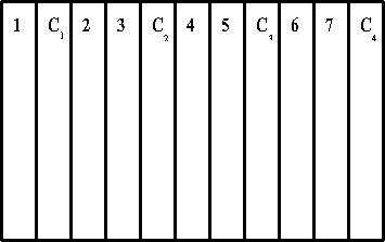
Figure 2 Replicated control design
The replicated control design is not a true statistical design for an applied research experiment. It will not conclusively show whether there are differences between treatments. Accepted statistical methods must be used to reliably show if and when treat ment differences truly exist.
Replicated Measurement t-Test Design
This type of design is well suited to field experiments when there is one treatment and a control condition, or two treatments. Suppose that you wish to find out if a new canola variety (A) is superior to an older, more commonly used variety (B). You want the study's results to apply across a region, so you recruit 20 farmers from across the region to participate in the study. Each farmer is prepared to plant either A or B in one field. The farms are then randomly assigned to A or B so that there are 10 f arms in each group. A simple way to randomly assign would be to put the farm names on a list, then take a deck of cards and pick out 10 hearts and 10 spades. Shuffle the deck of 20 cards, and then turn them over one at a time as you go down the list of names If a heart is turned over then the farm is assigned to variety A; if a spade is turned over then the farm is assigned to variety B.
When the crop yields have been determined (see Data Collection), the data can be analysed using an unpaired t-test. It is best to have between 10 and 20 observations (in this example, farms) for each treatment. Taking fewer than 10 observations makes it difficult to detect the systematic effects of the treatment.
A modification to the design that would improve the precision is the paired t-test. In this case each farmer provides two fields, and varieties A and B are assigned randomly to each pair of fields. This can be done by flipping a coin. As noted, this design's advantage is that detecting differences between varieties A and B is easier. The disadvantage is that it may involve more inconvenience to the farmer. The paired t-test is used when the design has been set up to link pairs of observations. Data may b e taken as paired when you can assume that sources of experimental error (factors that influence the outcome of the experiment that are not part of the treatment) are the same for each of the pairs. In this example it is assumed that factors such as soil fertility and moisture are more similar for fields on the same farm than they are for fields on different farms.
Figure 3 contrasts the differences between conditions for a paired and unpaired t-test analysis on two strips where each strip is about 0.4 ha (1 acre) in size. Results from both types of tests shown in Figure 3 would only allow you to generalize to the s trips as a whole.
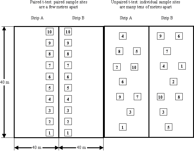
Figure 3 Plot designs for paired and unpaired t-test analysis
Often the research question involves more than two treatments (for example, three treatments and a control), but it is possible to locate the test strips in close proximity to each other in blocks so that the sources of experimental error are similar for the strips within a block. In this case the randomized complete block design is useful.
Randomized Complete Block Design
The randomized complete block design (RCB), shown in Figure 4, is widely used in field experimentation. It is an extension of the paired t-test. This design is appropriate when you are collecting quantitative data, such as yield, and you require a rigorous s comparison between treatments.
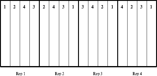
Figure 4 Randomized complete block design
The two cornerstones of the RCB design are replication (i.e., repetition) and randomization. These allow you to accommodate any variability in the local environment and to determine the probability of the differences in results between t treatments being real or simply due to chance.
Replicate each treatment a minimum of three times. Four replicates are better than three, and five better than four, but the statistical advantage gained is successively smaller with each added replicate. Replication locations must be selected to represent t the range of generalization.
Each treatment must be included once in each block of replications. The treatment locations must be randomly assigned to plots within the block. The purpose of randomizing the locations is to avoid biasing the results.
If field plots are your basic experimental unit, the individual plots should be three to five times long as wide and should be sized to comfortably handle one or two passes of the field equipment being used.
Proper plot location is important to reduce bias in the results. If the plots are on sloping land, run the long axis of the plots up and down the slope. With this layout, each plot will contain a portion of each slope position. (If the long axis of the plots runs across the slope, the lower slope treatment will be in a different environment than the upper slope treatment.) Similarly, if soil characteristics gradually change across the study site, run the long axis of the plots parallel to the gradient of soil variability. (See Site Location for more information on plot location.)
Two standard statistical tests are used together in analysis of data from an RCB design. An F-test, commonly called Analysis of Variance (ANOVA), is used to determine if there are significant differences between some of the treatments. If the F-test shows that significant treatment differences do exist, then a means comparison test, such as the Dunn's test or Duncan's Multiple Range (DMR) test, is used to determine which treatment means (i.e., treatment averages) are actually different f from one another.
There are two advantages to using an RCB design over the replicated measurement t-test design described above. One is the ability to compare numerous treatments using one analysis (the F-test). The second is the ability to separate out differences between replicates caused by environmental gradients (e.g., changing topsoil depth).
Split Plot Design
This design allows the testing of two factors in combination. One factor (the main effect) serves as a replication for the second factor (the split effect). There are many split plot design options, but the basic principle involves assigning one set of treatments to the main plots that are arranged in randomized complete blocks. The second set of treatments are assigned to subplots within each main plot.
An example of a split plot is shown in Figure 5. Six nitrogen treatments (A to F) form the main plots. Two sulphur levels (S1 and S2) form the split treatments and occur in each main plot.
The statistical analysis is similar to that used with the RCB design. That is, an ANOVA set up for a split plot is followed by a means comparison test such as the Dunn's test or DMR test.
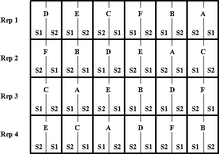
Figure 5 Split plot design
Factorial Design
In a factorial design, you can simultaneously observe the effect of two or more factors. That is, the design provides information on the average effect of the individual factors as well as the interaction between these two factors. For example, if nitrogen and sulphur fertilizers are the two factors being studied, you could determine if there was an additional effect of nitrogen and sulphur applied together that would not be accounted for by nitrogen or sulphur individually. This design type also allows a wider application of the conclusions reached on the effect of each factor because each factor is tested over a wide range of conditions of other pertinent factors. The statistical analysis used is ANOVA followed by a DMR test.
Figure 6 shows an example of a factorial design with two factors, canola variety and tillage system. The number of individual experimental units in each block is 15 (i.e., three tillage systems and five canola varieties). There are four replications, and the order of the experimental units in each replication is randomized.
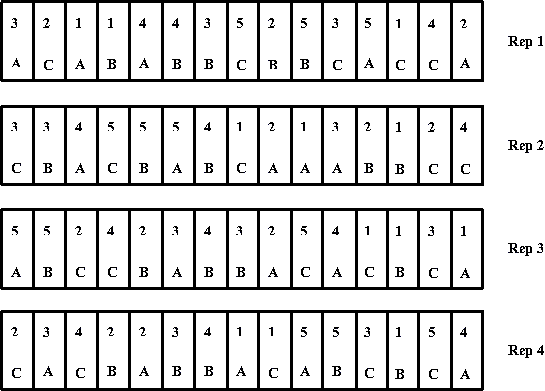
Figure 6. Factorial design consisting of five canola varieties (1,2,3,4,5) under three different tillage systems (A,B,C) |