| | Roles of Statistics in Agricultural Research
Agriculture and other life sciences consist of understanding the living world. Statistics promises carefully controlled acquisition of information for this understanding. Agricultural research is a complex process, but it typically consists of the following key steps:
- Formulate hypothesis and propose experiments;
- Identify appropriate experimental designs;
- Carry out the proposed experiments and collect data;
- Summarize the data and conduct appropriate statistical analysis;
- Evaluate the proposed hypothesis and draw conclusions.
Two of the five steps directly involve in the use of statistics. Thus, statistics plays an important role in biological and agricultural research.
So, to an agricultural researcher, what is statistics? In the narrow sense, statistics means an accumulation of facts and figures, graphs and charts, that is, any kind of factual information given in numbers. However, in the broad sense, statistics is the branch of applied mathematics that deals with data-based decision making. Therefore, statistics has two essential parts:
- Descriptive statistics: Collecting, organizing, presenting and analyzing data without drawing any conclusion or inference (e.g., drawing histograms from grouped data, computing mean, standard deviation, median and mode, etc.);
- Inferential statistics: This is the science of decision making in the face of uncertainty, i.e., making the best decision on the basis of incomplete information available from sample data or experimental data. Inevitably, uncertainty arises when we have only a sample taken from a population about which inferences are to be made. Thus, probability is important in the statistical decision making!!
Testing statistical hypothesis
Every research is carried out to test one or more hypotheses but not all hypotheses are statistical hypotheses. To be a statistical hypothesis, an assumption needs to be made about one or more parameters of a population (i.e., assigning a value to one or more parameters of the population). For example, the following statement is NOT a statistical hypothesis: Mars is inhabited by living beings, because it makes no assumption about one or more parameters of a population. However, the statement that Alberta's primary agriculture represents 22% of Canada's primary agricultural output is a statistical hypothesis because it assumes the proportion of primary agricultural outputs of different provinces and territories in Canada.
The test of statistical hypothesis consists of the following steps:
- Clearly state the null hypothesis (the hypothesis of "no difference") (H0). An alternative hypothesis (HA) must also be specified;
- Identify the test statistic, the value of which will be used to test whether to accept or reject H0. If H0 is rejected, we are left with the choice of accepting HA. NOTE: While we accept or reject a hypothesis, we have not proved or disproved it!!!
- Specify the decision-making rule. The null hypothesis is considered to be true if the calculated probability (based on the test statistic) is greater than the desired level of significance (
 ); it is considered to be false if the calculated probability is less than or equal to the significance level, and the result is termed significant. One has to make an arbitrary decision about the level of significance. It is commonly accepted that a result is considered to be significant if the calculated probability is less than 0.05. ); it is considered to be false if the calculated probability is less than or equal to the significance level, and the result is termed significant. One has to make an arbitrary decision about the level of significance. It is commonly accepted that a result is considered to be significant if the calculated probability is less than 0.05.
When we make a decision to accept or reject a hypothesis based on the results of an experiment (sample data), it is possible that we will make one of two types of wrong decisions:
 | True Situation |
Decision | H0 is true | H0 is false |
H0 is accepted | Correct decision | Type II error (  ) |
H0 is rejected | Type I error (  ) | Correct decision |
Clearly, Type I error equals to the level of significance ( ). The power of testing a statistical hypothesis is the probability that H0 is rejected given that HA is true, which is one minus the probability of Type II error = 1 - ). The power of testing a statistical hypothesis is the probability that H0 is rejected given that HA is true, which is one minus the probability of Type II error = 1 -  . However, the relationship between Type I error and Type II error is such that decreasing the probability of Type I error increases the probability of Type II error; Decreasing the probability of Type II error increases the probability of Type I error. This dilemma can be solved by (i) increasing sample size or (ii) using more efficient experimental designs or both. Thus, the experimenter has the direct or indirect control of both errors. . However, the relationship between Type I error and Type II error is such that decreasing the probability of Type I error increases the probability of Type II error; Decreasing the probability of Type II error increases the probability of Type I error. This dilemma can be solved by (i) increasing sample size or (ii) using more efficient experimental designs or both. Thus, the experimenter has the direct or indirect control of both errors.
Determining sample size: two treatments
The choice of sample size is a critical decision in any experimental design. Thus, statisticians are often asked: "How large a sample is needed for my experiment?" The question is not easy to answer! Before the statistician can provide anything better than an "educated guess", he/she must retaliate with several questions, the answer to which should enable him/her to attack the problem with some hope of reaching a valid answer. The following are a partial list of questions that the statistician may ask the researcher:
- What is your hypothesis? What are the possible alternative hypotheses?
- What are you trying to estimate?
- What significance level (
 ) are you planning to use? ) are you planning to use?
- How large a difference do you wish to be certain of detecting? With what probability (power = 1-
 )? )?
- What do you expect the variability of your data to be?
When the researcher provides answers to these and other questions, the statistician is able to help determine the needed sample size. In planning an experiment to compare two treatments, the following method is often used to estimate the size of sample needed. The experimenter first decides on a value that represents the size of difference between the true effects of the treatments regarded as important. The experimenter would like to have a high probability of showing a statistically significant difference between the treatment means. Probabilities or power (1 - ) of 0.8 and 0.9 are commonly used. A higher probability such as 0.95 or 0.99 can be set, but the sample size required to meet these severe specifications is often too large. The experimenter also needs to know population variance ( ) of 0.8 and 0.9 are commonly used. A higher probability such as 0.95 or 0.99 can be set, but the sample size required to meet these severe specifications is often too large. The experimenter also needs to know population variance ( ) or to guess it based on his experience. The formula for the needed sample size n is ) or to guess it based on his experience. The formula for the needed sample size n is
Here the two samples representing two treatments to be compared are assumed to be independent. For paired samples,  is replaced by is replaced by  , the population variance for the paired samples. This sample size is for a two-tailed test. If the test is an one-tailed test, the required sample size is calculated using the same formula except for replacing , the population variance for the paired samples. This sample size is for a two-tailed test. If the test is an one-tailed test, the required sample size is calculated using the same formula except for replacing  by by  . .
For easy use, one may want to tabulate the values of  for the commonest values of for the commonest values of  and and  . Evidently, these values are multipliers of . Evidently, these values are multipliers of  in paired samples and in paired samples and  in independent samples needed to determine the size of each sample. For example, if one wants the power to be 0.80 in a two-tailed test at 5% significant level, then in independent samples needed to determine the size of each sample. For example, if one wants the power to be 0.80 in a two-tailed test at 5% significant level, then  = 1.645 and = 1.645 and  = 0.842 and = 0.842 and  = (1.645 + 0.842)2 = 6.2. = (1.645 + 0.842)2 = 6.2.
Power (1-  ) | Two-tailed tests (  ) | One-tailed tests (  ) |
| 0.01 | 0.05 | 0.10 | 0.01 | 0.05 | 0.10 |
| 0.80 | 11.7 | 7.9 | 6.2 | 10.0 | 6.2 | 4.5 |
| 0.90 | 14.9 | 10.5 | 8.6 | 13.0 | 8.6 | 6.6 |
| 0.95 | 17.8 | 13.0 | 10.8 | 15.8 | 10.8 | 8.6 |
The same procedure can be used to calculate the sample size for comparing two proportions, p1 and p2. Here  = p2 - p1, and = p2 - p1, and  = p1(1-p1) + p2(1-p2). Thus, the formula for the needed sample size is, = p1(1-p1) + p2(1-p2). Thus, the formula for the needed sample size is,
For example, suppose that there is a new vaccine that is superior to the standard vaccine in reducing the mortality of young calves. A veterinarian wants to determine the sample size required for detecting a reduction from 2% to 1% of mortality with the power of 0.80 at the 5% significant level. The needed sample size is calculated as follows,
Thus, she needs 1829 animals for each vaccine.
Two scenarios may be particularly relevant: (i) the treatments are a standard and a new treatment hoped to be better than the standard; (ii) the experimenter intends to discard the new treatment if the experiment does not show it to be significantly superior to the standard. The experimenter does not mind dropping the new treatment if it is at most only slightly better than the standard but does not want to drop it on the evidence of the experiment if it is substantially superior.
When sample variance (s2) from the results of the experiments is used to be an estimate of  , t-tests replace the normal deviate Z-tests. However, the formula for n becomes an equation that must be solved by successive approximations. , t-tests replace the normal deviate Z-tests. However, the formula for n becomes an equation that must be solved by successive approximations.
Determining sample size: more than two treatments
Further complication arises when one wants to compare more than two treatments. Cochran and Cox (1957, p. 17-27) suggested the following formula to determine the number replications needed to detect the difference between pairs of treatments:
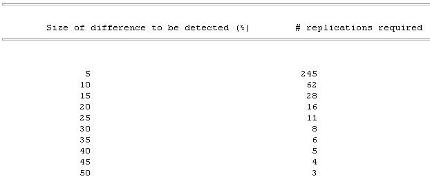
where CV is the coefficient of variation and  is the percentage of the difference of the mean to be detected. Let us consider an example to compute the sample size. is the percentage of the difference of the mean to be detected. Let us consider an example to compute the sample size.
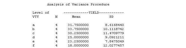
Example - An agronomist wishes to conduct a variety trial to compare the yield of six varieties of soybeans, A, B, C, D, E and F. Past experiments have indicated that an experiment in a randomized complete block design with four replications would be satisfactory for the proposed trial. She set up such an experiment and the following yields (seed yield in bushel per acre, 1 bushel/acre = 67.2 kg/ha) were recorded from her experiment. Does this experiment have a sufficient number of replications?
| Variety |
| Block | A | B | C | D | E | F |
| I | 42 | 42 | 41 | 25 | 31 | 36 |
| II | 33 | 37 | 33 | 27 | 16 | 12 |
| III | 31 | 37 | 33 | 35 | 29 | 11 |
| IV | 21 | 19 | 14 | 13 | 17 | 13 |
The desired number of replications (blocks) can be solved in iterative fashion. This means that we enter an initial value of n into the above formula and use it to obtain a better estimate of n.
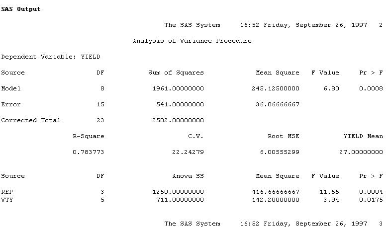
Initial conditions: The analysis of variance of the data gave the following baseline information needed to determine sample size.
First trial: We tried an initial value of n = 4 (4 blocks as in the original experiment) as a starting value. This gives us df = (6-1)(4-1) = 15 for the error term.
Second trial: Next we tried n = 16, making df = (6-1)(16-1) = 75 for the error term. Repeating the above calculation with this new df give us: n = 15. A further round was carried out and the same number was obtained. Thus, the desired number of replications is 15.
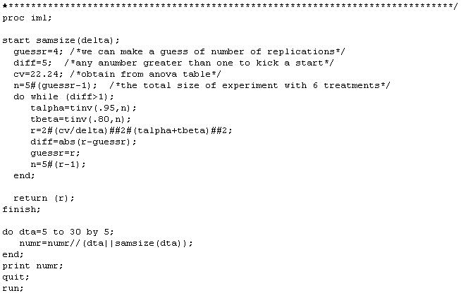
SAS Programs and Outputs for the above example
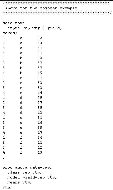
Calculate the number of replications required to detect the pre-set difference between pairs of means for the above RCBD design
(See Cochran and Cox 1957, Experimental design, p.17-23 for details)
Results from the above calculation
 |
|