| | Overview of SAS/STAT software | SAS Commands
Overview of SAS/STAT software
SAS/STAT software, an integral component of the SAS System, provides extensive statistical capabilities with tools for both specialized and enterprise-wide analytical needs. Ready-to-use procedures handle a wide range of statistical analyses, including analysis of variance, regression, categorical data analysis, multivariate analysis, and nonparametric analysis.
Analysis of Variance
Analysis of variance is a technique for analyzing experimental data. With SAS/STAT software, you can perform analysis of variance for balanced or unbalanced designs, multivariate analysis of variance, and repeated measurements analysis of variance. You can also fit general linear models and mixed models for a variety of data situations, including random effects, repeated measurements, and unbalanced designs.
Regression
Regression analysis examines the relationship between a response variable and a set of explanatory variables. The relationship is expressed as an equation that predicts the response variable from a function of the explanatory variables and a set of parameters. SAS/STAT software offers a general regression procedure that uses least squares to estimate the parameters, includes nine different model selection methods, such as stepwise regression, and produces a variety of diagnostic measures. More specialized procedures fit generalized linear models, mixed linear models, nonlinear models, and quadratic response surface models.
Categorical Data Analysis
Categorical data are those where the outcome of interest reflects categories, rather than the typical interval scale. The data are often presented in tabular form, known as contingency tables. With SAS/STAT software, you can investigate the association in a contingency table as well as produce measures that indicate the strength of that relationship. You can also use parametric models to investigate the variation of a function of the outcome variable across the various levels of the contingency table, analyzing functions such as means, logits, and proportions. Typical analyses include log-linear models, logistic regression, and bioassay analysis.
Multivariate Analysis
Multivariate analysis encompass a wide variety of methods for modelling data with two or more response variables or for identifying relationships among several variables without designating particular variables as response or explanatory variables. You can use common factor analysis to explain the correlations among a set of variables in terms of a limited number of unobservable, or latent, variables. Principal component analysis summarizes a large number of variables with a small number of linear combinations. SAS/STAT software also performs canonical correlation, discriminant analysis, path analysis, and structural equation modelling.
Nonparametric Analysis
Nonparametric analysis provides methods for analyzing data that don't require specific distributional assumptions such as normality. Many nonparametric methods are based on the ranks of the observations. SAS/STAT software performs nonparametric analysis of variance, including the Kruskal-Wallis, Wilcoxon-Mann-Whitney, and Friedman tests, as well as other rank tests for balanced or unbalanced one-way or two-way designs. Exact probabilities are computed for many nonparametric statistics.
Other Statistical Components in the SAS System
Several other components in the SAS System also provide statistical support. SAS/INSIGHT software is a highly interactive tool for data visualization and interactive data analysis. SAS/QC software provides tools for statistical quality improvement, including tools for statistical quality control and design of experiments. SAS/ETS software includes tools for econometrics and time series analysis. SAS/IML software is a powerful matrix-programming language with extensive mathematical operators and built-in functions that allow you to program statistical algorithms easily. SAS/OR software provides a wide range of optimization methods with numerous statistical applications.
SAS Commands
Most of statistical analyses encountered in agricultural research experiments are either analysis of variance (ANOVA), or regression analysis or combined ANOVA and regression analysis (i.e. analysis of covariance). In SAS, the main workhorse for regression analysis is proc reg, and for (balanced) analysis of variance, proc anova. The general linear model proc glm can combine features of both. Further, one can use proc glm for analysis of variance when the design is not balanced. Computationally, reg and anova are cheaper, but with the leap in desktop computing power in recent years, this is only a concern if the model has very many degrees of freedom (say, df > 500).
Analysis of Variance
Experiments involving a single factor or several factors with no missing data (balanced designs) can use the quick and easy proc anova to analyze the variation explained by those factors (analysis of variance, or ANOVA). More complicated ANOVA designs can be done PROVIDED the data are balanced. However, designs with imbalance among two or more factors should use proc glm.
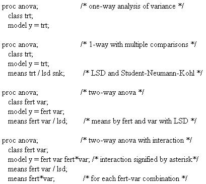
The class phrase is required, identifying all factors as categorical variables. The model phrase has only a few options, and these are not often used. The means phrase is quite handy to do multiple comparisons. Options Include:
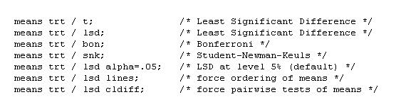
The lines to means option is default when data are balanced. The cldiff option can be useful at times, but it only gives differences CI for the differences, not the means themselves. None of these options works when looking at 2-way combinations such as means fert*var;.
If you want to save predicted values or residuals, or to evaluate contrasts, you must use proc glm instead of proc anova. See below.
Regression Analysis
Regression analysis is the analysis of the linear or non-linear relationship between one dependent (or response) variable and one or more independent (predictor) variables. Thus, the regression analysis basically carries out two major functions: (i) to establish the relationship between dependent and independent variables and (ii) to determine relative importance of each independent variable via assessing their contributions to the variation of the dependent variables.
(i) SAS commands to establish the relationship between dependent and independent variables
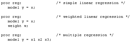
Here are simple uses of proc reg for standard problems:
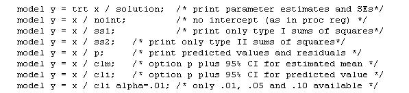
The model phrase indicates which variables are response (y) and which are predictors (x, or x1,x2,x3). Here are some print options for the model phrase:
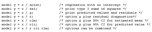
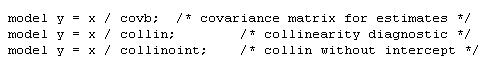
Here are some other model options for more advanced stuff:
The output phrase can have several keywords (which can be used together):
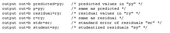
Only one output phrase can be used, but you can combine keywords on one line:

Those new variables created in set b are available for later plotting, etc.
(ii) SAS commands to determine relative importance of each independent variable
There is a stepwise model selection regression method. It works something like doing a series of proc regs, but the computer automatically makes the model choices of entry and elimination. Watch out! Be sure you know what this is doing for you (and to you).
proc stepwise;
model y = x1 x2 x3;
Here are model options for the means of selection and elimination:
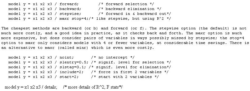
The significance levels slentry (or sle) and slstay (or sls) shown are the default ones (but sl=0.15 is used for selsection and elimination with stepwise option). The include option is useful if you want to force certain variables to always be in the model. The start option indicates how many must be in the model before elimination is considered (stepwise and maxr only).
General Linear Models (GLM)
The general linear models (GLM) procedure works much like proc reg except that we can combine regressor (continuous) type variables with categorical (class) factors. GLM Example: One-Way Analysis of Covariance is an example that illustrates the use of combined continuous variables and class factors. Under appropriate class and model statements, proc glm performs analysis of variance, regression, analysis of covariance and repeated measures. With two or more dependent variables in the data, it also performs multivariate analysis of variance. If your data are not balanced (i.e., unequal number of observations per cell and/or missing cells of class factors), then proc glm must be used to carry out the analysis of variance or analysis of covariance.
The organization of the printout is slightly different from reg and anova, and some model and output options are different. Further, if you want model parameter estimates, it is best to explicitly request the solution option in the model phrase.
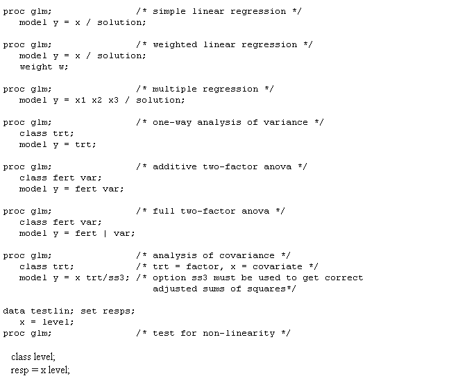
The class phrase works like in proc anova. However, here we can have both categorical (identified in class) and continuous variables in the model. The model phrase indicates which variables are response (y) and which are predictors (x, or x1,x2,x3). You won't get parameter estimates (solution) if there is a class phrase unless you ask for them. Here are some options:
The default way of estimating model parameters in SAS is to set the last group estimate to 0. Thus if there are 3 treatment groups, the estimated mean for group 1 is the intercept plus the estimate for trt=1; for group 2 it is similar; for group 3, the estimated mean for group 3 is the intercept since the estimate for trt=3 is 0. This can be changed by another option.
The means phrase works much the same in proc glm as in proc anova. Contrasts can be set up if means aren't enough. Here is an example from the glue data. The contrast phrase contains a quoted title, variable name and the contrast coefficient values. Note that the order of factor levels is lexicographic, which may not be what you expect. This can be checked by examining the order under the solution option to the model phrase. Further, these can get very complicated for higher order designs.
contrast 'A vs. rest' glue 1 -.25 -.25 -.25 -.25;
contrast 'BD vs. CE' glue 0 .5 -.5 .5 -.5;
Predicted and residual (and other) values can be passed to other procedures and data steps using the
output phrase in the same manner as proc reg.
Sums of Squares Types: I, II, III & IV
Issues of the choice of Sums of Squares arise with unbalanced designs including two or more factors or covariates. proc reg by default uses Type II sums of squares, while proc glm gives you Types I and III by default. There are four types of sums of squares (SS) available. Slight imbalance leads to slight differences in these SS, and hence in their tests. However, more severe imbalance can lead to fundamentally different conclusions (for rather different hypotheses)! Below are some notes; for more detail see Littell, Freund & Spector and/or Milliken & Johnson.
Short Summary of Types of Sums of Squares
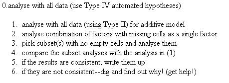
To examine these SS and associated tests, we must consider three experimental design scenarios (here a "cell" is a treatment combination):
1. balanced data (each cell has exactly r replicates)
2. unbalanced data but each cell has at least one observation
3. unbalanced data with one or more empty cells
WARNING: If you have (3) any empty cells, extreme care is needed to interpret ANY of the types -- get some help!!
All four types give the same results for scenario 1 (this is the same analysis as "proc anova"). For scenario 2, Types III and IV test the balanced hypotheses, while the hypotheses for Types I and II depend on the number of observations per cell. Here are the SS for a 2-factor design:
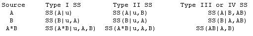
Type I (sequential)
incremental improvement in the error SS as each effect is added to the model
Type II (hierarchical)
reduction in error SS due to adding the term to the model after all other terms except those that contain it
Type III (orthogonal)
reduction in error SS due to adding the term after all other terms have been added to the model
Type IV (balanced)
variation explained by balanced comparison of averages of cell means
Type I SS have certain advantages: Hypotheses depend on the order in which effects are specified only for Type I. SS for all the effects sum to the model SS only for Type I SS. Type I SS for polynomial models correspond to tests of orthogonal polynomials. Type I SS are preferable when some factors (such as blocking) should be taken out before other factors, even in an unbalanced design.
Type II approach is appropriate for model building, and is the natural choice for regression.
Type III and Type IV tests differ only if the design has empty cells. SAS automatically gives you Types I and III with proc glm. You can explicitly choose types with options to the modelphrase:

Hypotheses for Unbalanced Data
With no empty cells, appropriate tests can be performed with Type III SS:
I/II
Hypotheses are functions of the cell counts (they differ from those tested if the data were balanced). This is usually undesirable. Type I hypotheses depend on order of terms in model.
III/IV
Hypotheses are the same for balanced and unbalanced data, involving simple, marginal averages of (population) cell means.
With one or more empty cells, main effects may not be what you think they are. Some marginal means are not defined. It is not generally obvious how to compare main effects.
I/II
Caution! Remember that hypotheses depend on cell counts.
III
Hypotheses do not depend on the order of effects or on the labels of levels. However, the orthogonal contrasts used are difficult to interpret unless you are willing to assume some interactions are zero.
IV
Hypotheses are balanced and easily interpretable. However, the SS may change if the labels of the factor levels are changed! Thus the exact tests performed depend on the order and labels of factor levels! Essentially, Type IV contrasts correspond to analysing subsets of factor levels chosen automatically.
What to do with empty cells? There is no easy answer to that one. My usual suggestion is something like this:
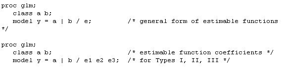
General Form of Estimable Functions
This is an advanced topic. The listings of estimable functions in SAS are rather confusing. It is strongly recommended that you read section 4.3.7 of the SAS System for Linear Models by Littell, Freund & Spector. The general form of estimable functions can obtained with options to the model phrase. Here are two examples:
|
|