| |
Foreword
This guide is designed to create awareness of the fundamentals of developing a water quality monitoring program with the primary focus on streams. It is intended for people interested in developing water quality assessment programs, such as applied researchers, technical specialists, agricultural fieldmen or watershed coordinators. The guide serves as an initial overview of water quality monitoring program design and tools to evaluate water quality. Readers are encouraged to consult additional resources including those listed in this document.
It is important to note that each situation requiring water quality monitoring is different and may require a different approach. Water quality monitoring is an expensive and time consuming endeavour requiring a substantial commitment of financial and human resources to obtain high quality, useful information. Consequently, program leaders, technical specialists and applied researchers are urged to contact water quality monitoring specialists to assist in individual program design and development.
Acknowledgements
The idea for this guide grew out of a 1996 workshop, sponsored by the Canada-Alberta Environmentally Sustainable Agriculture Agreement, on Agricultural Surface Water Quality Issues and Assessment Tools for Alberta Conditions. Alberta Agriculture, Food and Rural Development organized this workshop with participants from other government agencies, academic institutions and researchers from the United States Agricultural Research Service. The Alberta Environmentally Sustainable Agriculture Program supported the continued development of the information gathered from the workshop into this extension document.
Specific thanks go to A.-M. Anderson, T. Dietzler, S. Reedyk, D. Neilson, and J. Wuite for reviewing the guide, and to D. Fleury and B. Grinder for editing drafts of the guide. C. King was instrumental in getting this guide from draft to finished product.
Introduction
Agriculture, like other land uses, can affect the quality of surface and ground waters in Alberta. Protecting our water, land and air resources benefits the environment and the economy, and helps Alberta’s agri-food industry to produce high quality products in a healthy environment.
Studies in Alberta and elsewhere in North America clearly show that agricultural practices can negatively impact surface water quality (e.g. Anderson et al. 1998a; Anderson et al. 1998b; Cooke and Prepas 1998; Sosiak and Trew 1996; United States Environmental Protection Agency (USEPA) 1995). Impacts include increased nutrient and bacteria levels, and more frequent detections of commonly used pesticides in surface water samples.
With the recent heightened awareness of the effects that agricultural practices can have on surface water quality in Alberta, there is increased interest in undertaking water quality monitoring programs at a local level. However, water quality monitoring programs can be extremely time consuming and costly, and they tend to be data-rich and information-poor (Ward et al. 1986). This guide provides an introduction to developing a water quality monitoring program.
Objectives of this guide
This guide is for applied researchers, technical specialists or program leaders at the provincial or municipal level who wish to develop a water quality monitoring program. It introduces the key aspects of water quality monitoring, including defining program objectives, gathering appropriate data, and analyzing the data to adequately answer questions about water quality.
This guide is intended to create awareness about the fundamentals of water quality monitoring and the available assessment tools. It is not a comprehensive resource.
People interested in undertaking a water quality monitoring program are strongly urged to consult with water quality specialists or resource managers to assist with individual program development.
Fundamentals of Water Quality Monitoring
What is water quality monitoring?
Water quality monitoring is the integrated activity for evaluating the physical, chemical and biological character of water in relation to human health, ecological conditions and designated water uses (United States Geological Survey (USGS) 1995). It is a critical decision-support system for any water management program (USGS 1995). Information from a monitoring program can assist resource and program managers in making decisions or targeting community programming.
Monitoring requires the collection and interpretation of water quality data to provide information about water quality conditions. Those interpretations require additional information on hydrology, soils, land management activities and weather to make informed decisions to protect the quality of a water resource.
Setting monitoring program objectives
It is important to clearly state and understand the objective of a proposed water quality monitoring program before data collection begins. Identifying the objective assists in determining the experimental design and assessment tools that should be used in the program.
To determine program objectives, consider the questions that need to be answered with the monitoring results, the designated uses of the water resource, and the sources of contamination.
Possible objectives
Possible objectives for a water quality monitoring program include:
- preparing an impact assessment;
- forecasting ‘what if’ scenarios; and
- assessing the state of the environment, describing ambient conditions or identifying trends (USGS 1995).
Most of the monitoring in Alberta to date has been aimed at impact assessment. Impact assessments answer questions like: ‘What is the impact of livestock operations on the water quality in Pine Lake?’; and ‘What is the impact of agriculture on surface and ground water quality in the province?’
‘What if’ scenarios try to determine the changes that may or may not occur if a certain action is taken. ‘What would be the changes in water quality if a farmer moves his cow-calf wintering operation away from a creek draining to Pine Lake?’; ‘What would be the economic benefits and costs for the farmer?’; and ‘What are the water quality implications if cattle numbers double and hog numbers quadruple in Alberta?’ are examples of ‘what if’ questions.
State of the environment monitoring programs assess the ambient water quality at a watershed (drainage basin) or provincial scale. They attempt to measure whether our efforts are improving water quality, by assessing environmental indicators (e.g. the number of farmers making changes to their operations) and changes in water quality.
Designated uses and levels of protection
Designated uses of a water resource can include the following:
- drinking water;
- recreational uses and aesthetics;
- protection of aquatic life;
- agricultural uses (irrigation and livestock watering); and
- industrial supplies.
The designated use determines the level of protection required for the water source. Levels of protection are defined in a variety of ways including the following (Alberta Environment 1999):
- Guidelines - are recommended limits of parameters that will support and maintain a designated water use. They are given as numerical concentrations or narrative statements.
- Standards - are enforceable environmental control laws, set by a level of government. Standards are typically applied to effluent or emissions by industry to maintain a level of environmental quality.
- Objectives - are numerical concentrations or narrative statements that have been established to support and protect the designated uses of water at a specific site.
- Criteria - are scientific data evaluated to derive recommended limits of parameters for water use.
Compliance with water quality guidelines is the commonly used approach when evaluating ambient surface water quality in streams, river and lakes.
Canadian Environmental Quality Guidelines (as set by the Canadian Council of Ministers of the Environment (CCME) 2004) and Surface Water Quality Guidelines for Use in Alberta (Alberta Environment 1999) establish a framework for quantitative or qualitative measures of water quality indicators to support designated uses. More specifically, surface water quality guidelines are prepared for:
- protection of aquatic life;
- agriculture; and
- recreation and aesthetics.
A copy of the Alberta water quality guidelines can be found at the Alberta Environment website, or by mailing a request to:
Alberta Environment Information Centre
Main Floor, 9820 – 106 Street
Edmonton, Alberta T5K 2L6
The Canadian Environmental Quality Guidelines can be found at the Environment Canada website:
Sources of contamination
Understanding the contamination source(s) assists in developing an appropriate design for the monitoring program. There are two sources of contamination: point and non-point source pollution. In Alberta, agriculture can contribute both point and non-point source pollution.
Point source pollution- is the release of contaminants through the outlet of a single conduit, such as a pipe or ditch. Discharges into streams, lakes and rivers by wastewater treatment plants, paper mills, and other industrial facilities are classified as point sources of pollution. Runoff from a feedlot pen or overflows from a hog lagoon to a stream or lake are examples of agricultural point sources of contamination. Because point source pollution is usually concentrated, it is the most significant contamination source, but it is also the easiest to resolve. For example, runoff ponds or catch basins can be constructed to contain point sources.
Non-point source pollution - is pollution that does not originate from one location. Diffuse runoff from land and atmospheric-deposited pollutants not attributed to a single point of origin are considered non-point sources. Agricultural examples include runoff from agricultural land and water erosion from cropped fields. Controlling non-point source pollution tends to very difficult and usually requires a change in land management practices.
Water quality variables
Water quality is generally described according to biological, chemical and physical properties. Examples of different water quality attributes are listed in Table 1.
Table 1. Examples of water quality variables
Chemical | Biological | Physical |
Nitrogen (e.g. nitrate, nitrite, ammonia)
Phosphorus
Dissolved oxygen
pH (acidity, alkalinity)
Major ions (e.g. Ca++, Na+, Cl-)
Pesticides (e.g. herbicides, insecticides, fungicides)
Biochemical oxygen demand | Bacteria :�����Faecal coliforms
��������������������Total coliforms
��������������������Escherichia coli
��������������������Enterococci
Viruses
Parasites:�����Giardia
�������������������Cryptosporidium | Colour
Temperature
Odour
Total dissolved solids
Suspended solids
Turbidity |
Pollutants entering water bodies from non-point sources include sediment, nutrients such as nitrogen (N) and phosphorus (P) which are essential components of plant and animal diets, microorganisms from human sewage or animal manure, and pesticides used to protect crops from plant diseases, destructive insects and weed competition. Although most of these pollutants are transported in surface runoff, some may enter water bodies through atmospheric deposition, from direct application, or from sub-surface or shallow groundwater flow.
Sediment from field erosion fills streams, lakes and rivers and reduces their holding capacity. It affects the water’s capacity to sustain aquatic life by reducing light penetration and by altering bottom conditions. Sediment can also cause poor water quality because nutrients, organic matter and chemicals may be attached to the soil particles.
The major non-point sources of nitrogen include commercial fertilizers, animal manure, human waste and precipitation. Ammonia (NH3) and nitrate (NO3-) are the primary forms of inorganic nitrogen in water. Ammonia may be toxic to fish, depending on the acidity (pH) and temperature of the water. Although both are soluble in water, nitrates are more stable over a wider range of environmental conditions than ammonia. Nitrogen compounds, particularly nitrate, are highly mobile in soils and are easily leached past the root zone if in excess of crop demand. Nitrate can leach to and concentrate in shallow groundwater. High nitrate levels in ground water can be a potential human health risk by causing methaemoglobinaemia (or ‘blue-baby syndrome’) in infants (Mason 1996).
Non-point sources of phosphorus include commercial fertilizers, manure, and the minerals in rocks, sediment and soil. Phosphorus is less mobile in soils than nitrate, but can attach to soil particles. When these particles are deposited into water bodies, they can act as a long-term source of phosphorus. In Alberta, most of the phosphorus in runoff tends to be in the dissolved form (Anderson et al. 1998a, 1998b; Cooke and Prepas 1998). Dissolved phosphorus is more readily available for aquatic plant uptake, and excessive phosphorus in surface waters can trigger the rapid growth of algae and aquatic weeds (Sharpley et al. 1991). In turn, this can lead to eutrophication, or the accelerated aging of a lake. Eutrophication can result in fish kills due to low dissolved oxygen concentration, noxious tastes and odours, clogged water intake pipelines from algal matts and scums, and restricted use of the water body for recreation.
Disease-causing microorganisms (bacteria, viruses and protozoa) with the potential to affect human and livestock health, can enter surface waters in runoff containing animal or human wastes. Municipal discharges of sewage can also deliver bacteria and other organisms to surface waters. The application of animal manure and sewage sludge onto land should not be a significant non-point source of pollution, unless it is applied at excessive rates, in certain situations (e.g. winter spreading) or in locations with high runoff potential (Belsky et al. 1999).
Pesticides are compounds that do not occur naturally in the environment. Their presence in surface waters is the result of human activities. Pesticides can be carried in runoff, dissolved in water or attached to particulate material if they tend to persist in the environment and not break down. Pesticides can also enter surface waters by aerial deposition or by direct application onto surface water bodies. At high concentrations, they may cause health problems and even be toxic to all life forms.
Overall, excessive levels of nutrients, sediment, microorganisms and pesticides can make water unsuitable for human consumption, livestock watering and irrigation, and may pose a hazard to aquatic life. See Table 2 for examples of water pollutants and their implications.
Table 2. Some examples of water pollutants and their implications
| Pollutant | Primary Concern |
| Microorganisms | Public and animal health risk: water-borne diseases, livestock health |
| Nitrogen | Drinking water: high nitrates can be a risk to human health |
| Phosphorus | Protection of aquatic life: eutrophication |
| Pesticides | Protection of aquatic life; human health risk |
| Sediment | Protection of aquatic life; contaminant transport |
| Dissolved solids | Agricultural uses: salinity and livestock watering |
Variability in water quality
Aquatic ecosystems are dynamic systems and are influenced by many factors. Water quality monitoring to assess non-point source contamination in such ecosystems is particularly difficult because there is a large degree of natural variability to account for.
Factors contributing to variability in water quality data include:
- weather conditions;
- hydrologic conditions;
- sampling frequency;
- spatial variability;
- temporal variability;
- monitoring design;
- land use and land management practices; and
- analytical error (laboratory and statistical).
Weather conditions - Some water quality parameters may be positively or negatively correlated to weather conditions such as precipitation. For example, runoff from large rainfall events can pick up and deliver more contaminants to a stream than would be transported during dry weather. Conversely, some dissolved contaminants may not be affected by an increase in surface runoff or stream flow.
Hydrologic conditions and sampling frequency- Flow conditions in streams or seasonal influences on a lake affect water quality. To adequately characterize the quality of a water body, sampling must also account for the range of hydrologic conditions. Sampling streams infrequently or only during low flow periods will yield information that does not adequately characterize the stream’s overall water quality. Calculation of mass loads -- the total amount of a substance that is transported by a stream -- and flow-proportionate stream sampling -- taking more samples during high flows and fewer during low flows -- are required to describe ambient stream water quality.
Spatial variability- Spatial characteristics like sampling location can also affect variability in water quality. For example, water quality for certain parameters (e.g. dissolved oxygen, suspended sediment) may differ depending on whether the sample was taken at the surface or bottom of a stream. Variability may also be introduced if a sampling station was changed between years.
Temporal variability- The time of day (daily) or the time of year (seasonal or annual) when samples are taken can influence the concentration of a particular water quality variable, such as dissolved oxygen.
Monitoring design- The type of sampling (i.e. grab or composite samples) is another way variability can be introduced into a sampling program. Grab samples are discrete samples that are taken at specific sampling times. Composite samples are samples taken over a period of time (e.g. hours or days) or from a variety of locations and combined into one sample.
Land use and land management practices- A long period of record is required to determine if change or level of impact is due to the effects of a particular practice or to natural variability. Consequently, a long-term commitment is recommended to adequately assess water quality.
Analytical error- Laboratory analysis can also introduce a level of variability or error into water quality data. Quality control and quality assurance components, to validate the data, should be part of any water quality monitoring program (see Quality Control and Quality Assurance section for more details). Statistical analysis tests (e.g. analysis of variance, t-test) can also introduce a certain level of error into the evaluation of water quality data.
In general, there is a large amount of natural variability in the quality of water resources. To determine statistically significant differences in water quality or to properly characterize the water quality of an aquatic system, data from several years are recommended to account for this natural variability.
To aid in explaining variability in monitoring results, it is imperative to document sampling protocol (e.g. grab or composite sample) and describe conditions at the sampling sites (i.e. verbal descriptions of weather conditions, the overall state of the stream, etc.).
Designing a Water Quality Monitoring Program
Once the program’s objectives, designated uses of the water body and possible sources of contamination are clearly identified, then program developers can begin to consider the program’s experimental design or approach. The program design should consider: which water quality variables need to be measured; what additional information is needed; what experimental design will best answer the questions that need to be answered; what budget and manpower are available; and how to ensure high quality data.
Selecting water quality variables
Water quality variables to be evaluated in a monitoring program should be selected according to:
- the program’s objectives;
- the designated uses of the water body being monitored;
- the land management activities being evaluated; and
- the budget and manpower allocated for the program.
For example, a water quality monitoring program is proposed to evaluate the impact of a livestock operation on a downstream lake. This program would include water quality variables characteristic of livestock operations and applicable to aquatic ecosystems. Phosphorus and nitrogen are found in animal manure and can impact water quality in lakes and therefore should be included in the monitoring program.
However, simply monitoring for nitrogen and phosphorus downstream of any livestock operation is not sufficient to determine cause-and-effect relationships, as both phosphorus and nitrogen can be attributed to other sources. Other variables, such as stream flow, precipitation and land use information (e.g. livestock or manure management practices) must also be evaluated to determine which factors are linked to the change in water quality.
Other required information
Before starting a water quality monitoring program, it is important to collect appropriate supplementary information to account for sources of variability in water quality. Accounting for most of the major sources of variability increases the likelihood of identifying the effect of a particular land use or management practice on water quality.
Additional information needed for a successful monitoring program includes:
- stream discharge and other hydrologic variables;
- climatic and seasonal variables;
- agricultural practices (e.g. livestock density, cropping patterns, timing and application rates of fertilizers or pesticides); and
- soil, vegetation, geology and topography characteristics.
Hydrological data such as stream flow are essential to evaluate surface water quality. The sensitivity to detect changes in water quality as well as attribute water quality changes to specific land use practices is much lower when stream flow is not recorded during a water quality sampling program (Spooner et al. 1985).
Stream flow represents a watershed’s response to climatic conditions, especially precipitation. Ideally, each stream site being monitored should have an active stream flow gauging station. Statistical summaries of historical stream flows and associated return periods from rainfall events are also beneficial to put each monitoring year into context. This information helps to characterise the watershed’s response to precipitation and will assist in determining sampling frequency. Water Survey of Canada has a network of hydrometric stations across Alberta that measure continuous stream flow of selected streams and all major rivers.
Stream discharge is the rate of stream flow expressed in volume per unit time. Stream discharge can account for much of the variability in water quality data. Thus, it is very important to collect stream flow data from an established stream gauging station and to establish the relationship between stream stage (the height of the water surface, measured by the stream gauge) and stream discharge. For example, a greater amount of phosphorus tends to be delivered during periods of high stream flow. If stream samples are collected randomly without any information on stream flow, the water quality in the stream cannot be fully characterized and the information generated from such a sampling program is limited.
Stream discharge is a critical explanatory variable for quantifying the mass load of pollutants being delivered from a watershed (see section on Calculating Mass Loads). Therefore, conducting flow-proportionate sampling or sampling during the range of stream flows for a particular stream or river system is recommended for all monitoring programs.
Surface runoff is the main mechanism for transporting non-point source contaminants from the land to surface waters. Runoff is a complex function of many factors including precipitation, infiltration and vegetation. Infiltration depends on soil attributes such as texture, structure and depth of the soil horizons. These parameters determine the soil’s water-holding characteristics and tendency to erode. Vegetation plays an important role by intercepting rainfall, retarding runoff and enhancing infiltration. Topographic factors such as slope and surface depressions determine flow velocity and surface storage. Geology controls percolation and ground water seepage, and the mineral content in surface and ground waters. Information on these characteristics assists in qualitatively explaining the results of a monitoring program.
The extent of land contributing to stream flow, called the effective watershed area, is also important. This is particularly so in the prairies, where potholes, wetlands and sloughs affect the quantity, and possibly the quality, of water reaching watershed outlets. Areas that do and do not contribute water to the stream flow must be properly mapped to obtain accurate estimates of the effective drainage area. Otherwise the amount of runoff and pollutant loadings can be under- or overestimated. It is also important to note that the effective watershed area is highly dependent on climatic conditions, and it may change from year to year.
Required climatic information includes rainfall intensities (i.e. the rate at which rain falls), storm durations (i.e. the length of time of a rainfall event at a certain intensity) and temperature fluctuations (Satterlund and Adams 1992). Data obtained from on-site or off-site stations must capture the variability of climatic conditions in the watershed, including information on both extreme and average conditions. Other important weather variables include diurnal (i.e. daily) temperature fluctuations, wind velocity and solar radiation. These data are particularly useful in computer models to estimate other meteorologic information like evaporation/evapotranspiration and forecast ‘what if’ scenarios.
Information on agricultural management practices must also be collected. Tillage type, the amount and type of fertilizer or pesticide, application method, application timing (especially with respect to subsequent rainfall or irrigation events) and other practices can affect both the quantity and quality of surface runoff. For example, reducing tillage may reduce soil loss, but may increase the availability of dissolved nutrients and pesticides to be transported in runoff (Alberts and Spomer 1985).
Historic water quality data, where available, are extremely useful to characterize previous water quality conditions. However, the quality of the data may be suspect if analytical methods have changed with time.
Experimental design
The experimental design of a monitoring program must be developed to meet the program’s objectives. If the experimental design is not adequately developed before data collection begins, the program’s objectives may not be met. The design must specify the type and number of water quality attributes being monitored, number of monitoring stations, and the sampling frequency to effectively characterize water quality for the purposes of the program.
In general, water quality monitoring program designs can be categorized in four ways:
- single point (i.e. stream mouth);
- upstream/downstream;
- before/after treatment; and
- paired watershed.
The program’s objectives determine which experimental design is most appropriate. For example, monitoring at a single site, such as the stream outlet, may be adequate to broadly characterize the water quality of a particular watershed. However, if the objective is to assess the impact of a specific agricultural activity (e.g. a feedlot that builds a manure runoff catch basin) on water quality, then an upstream/downstream or before/after design is more suitable.
A paired watershed design is used to assess two or more watersheds with similar hydrological, climatological and land attributes, that differ in a single characteristic to be evaluated, such as land cover, number of feedlots or tillage practices. One of the watersheds is the control or reference watershed; the other watershed has the treatment (the practice or characteristic being evaluated). The control watershed is used to characterize the year-to-year variability. Thus, the differences between the treatment watershed and the control can be attributed to the treatment rather than to other variables like weather or runoff volumes.
Monitoring programs need to be conducted over a sufficient amount of time (i.e. years) to characterize the natural variability (e.g. climatic variability due to differences in runoff from snowmelt or rainfall). In some instances, five or more years are required to define impact or determine if a change in land management contributes to a change in water quality. For example, to quantify the changes in water quality produced by changes in land management practices, two or three years of initial monitoring are recommended to characterize the water quality and natural variability of the watershed before any change to land management practices. Once the new practice has been implemented, a further two to three years are recommended to determine if any significant change in water quality has occurred.
Shorter time frames can be used to identify specific water quality impacts. Upstream/ downstream monitoring over one year may be able to show a significant difference if a lot of thought is put into the sampling design.
Please refer to Spooner et al. (1985) for a thorough discussion on the advantages and disadvantages of different monitoring designs.
Budget
A substantial commitment of manpower and equipment is needed to conduct a monitoring program to obtain sound scientific information on the quality of a water resource. Consequently, the budget may be the most limiting factor in a water quality monitoring program’s development.
Money and time must be allocated to:
- equipment, taking into account the number of monitoring stations needed;
- sample collection, taking into account the frequency of sampling needed to characterize the range of conditions (e.g. peak flow and base flows);
- transportation of samples and manpower to and from the monitoring stations; and
- analytical costs, taking into account the type and number of attributes being sampled.
If hydrometric equipment is already in place (i.e. Water Survey of Canada gauging stations), then manpower and analytical costs will be the most limiting factors. Automatic water samplers, continuous stage recorders and current meters may be expensive, but are usually a one-time cost. Other budget commitments will depend on the length of time needed for the monitoring program.
Quality control and quality assurance
Many factors can introduce error into a water quality monitoring program. Therefore, it is very important to implement a rigorous quality control (QC) program to check the quality of the data being collected. Quality assurance (QA) is an integrated system of management procedures and activities used to evaluate data quality and verify that the QC program is operating within acceptable limits (USEPA 1997). Such a program is essential for the collection of scientifically sound water quality data.
A QC/QA program usually incorporates the collection and analysis of blank, duplicate, replicate and/or spiked samples, reference materials to ensure the integrity of the analyses, and regular inspection of the equipment to ensure it is operating properly.
Factors such as improper sampling protocol, careless laboratory analyses, contamination from improper handling of water samples, and imprecise monitoring equipment can compromise the quality of the data and the subsequent information gained from a monitoring program. It is also important to check the laboratory’s method detection limits for the selected water quality attributes. If the method detection limit is higher than the level required by the monitoring program, then the data from the laboratory may be useless.
Other QC activities may include regular calibration of sampling equipment, regular inspection of reagents used for contamination analyses, and regular checking of laboratory support equipment (e.g. drying ovens, refrigerators, etc.).
Water Quality Assessment Tools
Empirical methods and computer simulation models are the two most common tools used by resource managers to interpret data for water quality assessments. Although these tools can be used independently, usually a combination is used. For example, past and existing trends can be interpreted from water quality monitoring data, but the susceptibility of the environment to weather events other than recorded storms would have to be modeled. Examples of different assessment tools are given below.
Empirical methods for data analysis
Empirical methods involve field measurements of water quality. Data collected from a monitoring program may typically be:
- displayed graphically;
- compared with water quality guidelines;
- used to calculate mass loads, export coefficients and/or flow-weighted or time-weighted mean concentrations; and/or
- evaluated statistically to determine significant differences and similarities.
Graphical techniques
Displaying data in graphs allows for more effective visualization of the data and more effective presentation of large data sets in a small space. Graphical presentations capture the attention of readers and assist both the reader and the data analyst to see:
- problems or gaps in the data;
- relationships between variables; and
- trends in selected water quality variables.
Graphical methods, such as the use of time-series plots, histograms, x-y graphs, box-whisker plots and pie charts, are fundamental tools used in water quality assessments. Geographical information systems (GIS) present data in a graphical format that conveys the spatial distribution of water quality data.
A time-series plot displays the data for one or more water quality variables against the sampling date (time) and shows the temporal variability in water quality attribute concentration or stream flow (Figure 1). It helps in visualising changes over time, potential trends or seasonality, cyclic variations, and extreme values or outliers. Outliers or extreme values are data that do not conform to the rest of the data in a particular database. Unless outliers can be traced to errors due to sampling or laboratory analysis, etc., these data are meaningful and must be included in any data analysis.
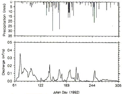
Figure 1. Example of a time series graph .
A box-whisker plot (Figure 2) can illustrate both the distribution and summary statistics of a data set. The box in a box-whisker plot shows the 25th and 75th percentile of the data set, called the lower and upper quartiles, and the median (the 50th percentile) (Mendenhall 1987). The ‘whiskers’ extending vertically from the box represent the range of the data set, usually the maximum and minimum values. Extreme values can also be plotted on the graph using separate symbols, such as asterisks or daggers.
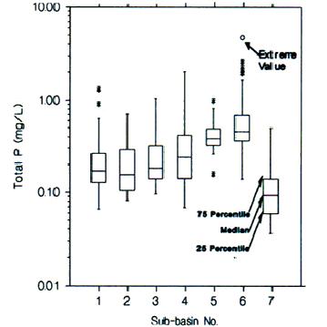
Figure 2. Example of a box and whisker graph (data from Sosiak and Trew 1996) .
Another graphical tool used to compare grouped levels of water quality data is the bar chart or histogram (Figure 3). Bar charts are commonly used to illustrate the differences between events, sites and treatments affecting water quality. Bar charts can convey the variation in the mean or median values of water quality parameters, by including error bars such as the standard error of the mean, or standard deviation.
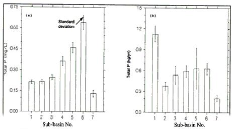
Figure 3. Example of a bar or histogram chart showing the standard deviation.
Some graphical procedures (e.g. the presentation of box-whisker plots, normal probability graphs, and the use of smoothing functions) assist investigators in the interpretation of information contained in the collected data. These procedures combine the use of graphical and statistical methods in one plot.
The use of graphical tools is an exploratory procedure, serving as a stepping stone for further analyses to answer specific water quality questions. These exploratory methods are key to selecting the most appropriate tools for further assessment and therefore should be used before other types of analyses.
Compliance with water quality guidelines
Alberta Environment has developed Surface Water Quality Guidelines for Use in Alberta (Alberta Environment 1999) to provide general guidance in evaluating surface water quality throughout Alberta. Surface water quality guidelines have been developed for the protection of aquatic life, agricultural uses, and recreation and aesthetics. The Canadian Environmental Quality Guidelines (CEQG) for water are user-specific guidelines for the protection of recreation, aquatic life, community water supplies and water for agricultural uses (CCME 2004).
Water quality guidelines may be applied to the evaluation of runoff samples, but it should be recognized that the guidelines were established for lakes and larger rivers. Thus, these guidelines may not always be directly applicable to surface runoff or even small streams. Nonetheless, they can be used as a cursory measure for evaluating water quality.
Water quality data that fall between the range of recommended values outlined by the guideline for a particular use are considered compliant. Generally, for a defined period of record (e.g. annual) as outlined by the monitoring program, the compliance frequency or the ratio of samples meeting guidelines to the total number of samples taken, is reported (Anderson et al. 1998a). The minimum - maximum concentration range and the average amount by which samples exceed guidelines, can also be relative measures of the degree of non-compliance.
Some water quality guidelines provide a relative threshold, such as an increase in concentration above background levels. The definition of background level is critical. Background levels may be defined by sampling a reference or control site, or by comparing paired samples, such as upstream and downstream samples. If downstream concentrations do not exceed upstream concentrations, or if a study site does not exceed the concentrations found at a control or reference site by the amount defined in the guideline, the concentration is considered to be compliant. (Details on the use of water quality guidelines for compliance analyses are given in Anderson et al. (1998a).)
Calculating mass loads
The calculation of the total mass load of a contaminant being carried in a stream assists in determining the magnitude of impact on a downstream water body. Mass load is a calculation of the total mass of a substance, usually expressed in kilograms, that is carried past a particular point on a stream or river for a given time period (e.g. year).
To calculate a mass load of a substance, an estimate of stream flow must be taken concurrently with water quality samples. In a flow-proportionate sampling program, an individual water sample does not characterize the stream for equal lengths of time. Therefore, to estimate the average concentration, each sample has to be weighted according to the length of time it is used to represent the stream system (Baker 1988).
Thus, mass load is the sum over a particular time period (e.g. month or year) of each sample’s concentration multiplied by the instantaneous stream flow rate when the sample was taken, multiplied by the length of time that the sample represents (Equation 1):
Mass Load = Σ ci qi ti �������������������������������������������������������������������������������� Equation 1
where �� i = 1 to n (number of samples)
������������ ci = samples concentration (mg/m3)
������������ qi = instantaneous stream flow (m3/sec)
������������ ti = time interval (seconds)
The time interval is equivalent to one-half of the time interval of that sample and the preceding sample, and one-half of the time interval between that sample and the following sample. Computer programs (e.g. FLUX 5.1 (Walker 1996)) can be used to automatically calculate total mass loads.
Pollutants from non-point sources tend to be delivered during periods of high stream flow. Consequently, a flow-proportionate sampling program must be used to obtain accurate estimates of total mass load of a pollutant.
Calculating mass export coefficients or unit area loads
The total mass export coefficient or unit area load is the estimate of the amount of contaminant lost per acre or square kilometre of watershed. Export coefficients are calculated by dividing the total mass load (see above) of a substance by the watershed area (actual or effective drainage area) upstream of the sampling station for a given period of time (e.g. year).
Mass Export is defined as:
Mass Export = ����� ������� Mass Load (kg)������������������������������������������� ��������������Equation 2
����������������� ��������������Watershed Area (km2)
The calculation of mass export coefficients (as kg� km-2 � yr -1) allows for general comparisons of pollutant export from watersheds with differing sizes. However, export coefficients are strongly influenced by runoff volume due to climatic factors, and pollutant delivery of different water quality parameters may behave differently depending on watershed size or scale. Thus, comparisons between watershed export coefficients may be more qualitative than quantitative.
Export coefficients also quantify how much of a substance is leaving a particular area. Export coefficients on nutrient loss from a field, for example, illustrate how much fertilizer may be lost from a farming operation. These export coefficients can be used with cost estimates for nutrients to see whether the loss is economically significant to the farmer.
Calculating flow weighted mean concentrations
Flow weighted mean concentrations (FWMC) are concentrations that are adjusted for the variability in stream flow over a given period of time (e.g. monthly or annually). FWMC is useful for estimating the typical concentration of a contaminant adjusting for stream flow. This allows for comparisons between streams with different flows or between years when a stream has different flow volumes.
FWMC is defined as :
FWMC = ����� ������� Total Mass Load (kg)������������������������������������������� ��������������Equation 3
�������� ��������������Total Stream Flow Volume (m2)
where the total mass load (kg) is divided by the total stream volume (m3) for a given time period (e.g. year or month). By calculating FWMC on a monthly or annual basis, variability due to seasonal and historical sampling frequency fluctuations and missing data can be reduced. This also reduces the range of the data and makes it more manageable (Richards and Baker 1993). For an example of calculating a FWMC, see the box below.
Example calculation of total mass load, total export coefficent and flow weighted mean concentration
A | B | C | D | E | F | G | H |
Sample
Number | Time of
Sample | Seconds
between
Samples * | Stream Flow
(m3/sec) | Total
Stream
Volume (m3)** | Total
Volume (L) | Phosphorus
Concentration
(mg/L) | Phosphorus
Mass Load
(mg )^ |
1 | 930 | 5550 | 0.005 | 27.75 | 27750 | 0.156 | 4329 |
2 | 1235 | 9450 | 0.010 | 94.50 | 94500 | 0.210 | 19845 |
3 | 1445 | 6150 | 0.009 | 54.74 | 54735 | 0.056 | 3065 |
4 | 1600 | 7650 | 0.005 | 34.43 | 34425 | 0.075 | 2582 |
5 | 1900 | 5400 | 0.004 | 18.90 | 18900 | 0.050 | 945 |
TOTAL |  | | ---- | | 230310 | ---- | 30766 |
*��� assuming 930 am is the start time and 1900 is the end of the sampling program
**� column C multiplied by column D
^��� column F multiplied by column G
The total mass load of phosphorus (mg) is equal to the sum of column G = 30766 mg or 30.77 kg.
The Flow Weighted Mean Concentration of example in the table above is:
FWMC = ����� �� Total Mass Load ������������ = �������������� � 30,766 mg �������������� = ������� 0.136 mg/L
�������������� ��������� Stream Volume �����������������������������������230,310 L
This differs greatly from the arithmetic mean that does not consider the variation of stream flow of 0.109 mg/L.
The export coefficient would be the total mass load divided by the hypothetical watershed area. For example, if the hypothetical watershed area were 10 km2, the export coefficient would equal the total mass load divided by the watershed area:
Export Coefficient = �� �� 30.77 kg ������������ = �������������� 3.08 kg/km2 (for sampling time period)
�������������������������������������� 10 km2
The sampling time period for this example would be less than one day; however, export coefficients are usually computed for an entire year.
|
Statistical methods
Statistical methods are basically mathematical models used for identifying the effect of single or several water quality variables. Statistical methods may address whether water quality indicators at a given site meet guidelines, whether there has been a significant change in water quality between sampling sites or time periods, or whether water quality for a designated use is being affected. An excellent summary of statistical tools applicable to hydrology and water quality is contained in chapter 17 of the Handbook of Hydrology (Maidment 1993) and Statistical Methods in Water Resources (Helsel and Hirsch 1992).
Statistical methods frequently used for water quality assessments include descriptive statistics, hypothesis testing, regression analyses, and time-series analyses. Some of these empirical methods can be done by hand if data sets are small or if summaries of data are available. However, computer spreadsheet programs or statistical programs should be used when data sets are large.
Descriptive statistics
The mean and standard deviation are important statistical indicators. Knowledge of the mean and standard deviation is necessary for calculating skewness and kurtosis coefficients, which are indicators of the data distribution. However, water quality data tend to have non-normal distributions and contain a significant amount of variability. Consequently, the median or the middle measurement of a data set (Zar 1984) can be used to describe the data set.
The relationships between variables in a data set can be obtained from correlations. Correlations relating numerical data, such as discharge (x) and phosphorus concentrations (y), can be calculated from the use of Pearson’s correlation equation. Please refer to statistical textbooks like Maidment (1993), Helsel and Hirsch (1992) or Zar (1984) for more information.
Parametric vs non-parametric methods
Use of parametric statistical methods, such as regression equations and analysis of variance (ANOVA) tests, requires that the two (or more) sampled populations be normally distributed and have equal or similar variances. Using parametric tests for data sets that depart from normality could lead to erroneous conclusions.
Non-parametric tests or transformation techniques are used when data are not normally distributed and the variances are not homogeneous. Non-parametric tests are considered ‘distribution-free’. The most common transformation method for water quality data is the use of logarithmic transforms: x = ln(x). Other transformations can be used to remove trends or variability in the data set due to other factors that may be affecting the data.
Parametric tests are often more robust and powerful than non-parametric tests; however, non-parametric tests must be used when the data do not meet the criteria for parametric tests.
Testing for normality
Data sets must be tested for normality to determine whether parametric or non-parametric tests are appropriate. Tests for normality include:
- using graphical tools such as histograms (Figure 4) or normal probability plots (Figure 5);
- computing the skewness and kurtosis coefficients of data and testing their departure from normality; or
- using statistical tests such as the Kolmogorov-Smirnov goodness-of-fit test.
Non-parametric methods
Water quality data sets tend not to have a normal distribution or homogeneous variances. Therefore, most water quality data sets require non-parametric statistics to evaluate and test hypotheses.
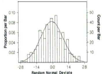
Figure 4. Typical histogram of normally distributed data
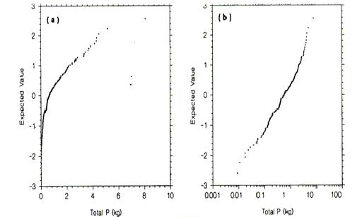
Figure 5. Example of normal probability plots of total phosphorus on original data (a) and log-transformed data (b)
Commonly used non-parametric tests include the following:
- Kruskal-Wallis test;
- Mann-Whitney test;
- Kolmogorov-Smirnov test;
- Lilliefors test;
- Sign test;
- Wilcoxon Rank Sum test; and
- Wald-Wolfowitz test
For example, a Kruskal-Wallis test is used to determine if total phosphorus loadings from several land uses (e.g. forest, pasture, crop land and urban) are statistically different. This test is analogous to the parametric one-way ANOVA test. The Mann-Whitney test determines the difference between only two treatments, which is similar to the parametric Student’s t-test. Kolmogorov-Smirnov test is used to compare the differences between the cumulative distributions of two samples. For example, nitrite-nitrate data from a watershed can be compared to that from a similar watershed in a different region, or can be compared to a random sample generated from a normal distribution to determine if data are normally distributed.
Anderson et al. (1998a) and (1998b) are excellent studies that illustrate the use of non-parametric statistics for water quality data. For more information on non-parametric statistical analysis, please consult statistical textbooks like Conover (1980) and Helsel and Hirsch (1992).
Regressions
Regressions relate a dependent variable, such as total phosphorus, to one or more independent variables (e.g. discharge). There are two types of regressions:
- linear (e.g. y=b+mx)
- non-linear (e.g. z=a+b/w+cex+dy3; where w, x, and y are independent variables)
Linear regression is the most common type used for water quality data analysis. However, the application of linear regression requires normally distributed data. If data are not normally distributed, then one must use data transformation techniques or non-linear models.
Regressions not only show the relationships between independent variables and their dependent parameters. They are also essential for:
- estimating missing data (e.g. infrequently sampled water chemistry data at a site where continuous discharge is monitored);
- relating water quality data from sites with similar characteristics; and
- generating input data for water quality models.
A scatter plot showing the linear association between discharge and total phosphorus is presented in Figure 6. The use of log10 scales in Figure 6 is an indicator of the need for a transformation of original data to fit a significant (i.e., P<<0.0001) regression equation with high coefficient of determination (r2=0.862; transformed data). To ensure that the residuals are normally distributed and do not follow an identifiable pattern, it is necessary to perform diagnostic checks similar to those in Figure 7.
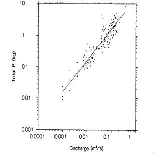
Figure 6. Relationship between discharge and total phosphorus, with regression line fitted to data
Figure 7. Graphical depiction of diagnostic checks performed on the residuals of regression line plotted in Figure 6
Mathematical time-series analyses
Mathematical time-series analyses can be used to relate the value of a variable at a given time to historical data. In water quality assessments, time-series analyses are usually used for prediction of missing data or for forecasting.
Auto-regressive integrated moving average (ARIMA) analyses are the most common time-series analyses employed in water quality investigations (Hipel and McLeod 1994). Simple auto-regressive analyses have been used for the prediction of rainfall events. Moving average analyses were found useful in the prediction of daily temperatures. Recent introductions include intervention methods that are used for comparing before and after conditions, or for testing changes due to treatment effects or regulatory actions.
For more information on the use of time-series analyses in water quality investigations, please refer to statistical texts or Hipel and McLeod (1994).
Water quality simulation models
Computer models are frequently used in water quality assessments, especially when objectives include risk assessments, change detection or data augmentation. Water quality simulation models may consist of several types of sub-models, such as empirical and physical equations. Models differ by the methodology and scale by which system parameters are represented.
Agricultural water quality models usually fall into the following categories:
- lumped, where an area of interest is treated as a single homogeneous entity;
- spatially distributed, where a basin is subdivided into a number of small heterogeneous sub-units with dissimilar attributes;
- single event or continuous time; and
- field or watershed scale.
Models could also be classified as either deterministic, where everything is known, or stochastic, where only probabilities are known.
Donigian and Huber (1991) describe non-point source pollution models applicable to non-urban environments. They also provide detailed information on the requirements of several watershed scale models including Agricultural Non-point Source Pollution Model (AGNPS) (Young et al. 1989) and Simulator for Water Resources in Rural Basins (SWRRB) (Arnold et al. (1990)).
The Soil Water Assessment Tool (SWAT) is an improved version of SWRRB that can easily be coupled to the computer model GRASS GIS (Srinivasan et al. 1993). The improvements in SWAT over SWRRB include:
- simultaneous simulation of up to 2500 sub-watersheds;
- enhanced ground water simulation of both lateral flows and shallow aquifers;
- advanced reach routing;
- simulation of sediment and chemical movement through ponds, reservoirs and streams (Srinivasan and Arnold 1994); and
- although the model still lacks a feedlot simulation component, it can be linked to a new model, APEX, to simulate point sources of pollution.
To use water quality models for assessment, one must examine the suitability of the model for meeting the objectives of the assessment, whether the input data required by the model could be obtained, and if the model output can be evaluated by comparing it to observed data.
Suitability of a water quality model also depends on how it represents the spatial and temporal properties of water quality parameters of interest. The model should approximate both the scale and the processes that affect water quality in the study area. Input data should quantify the conditions at the study area during the water quality investigation. If some of the input requirements are not available, they must either be collected in a monitoring program specifically designed to meet the objectives of the modeling project, or values must be estimated from existing literature. The implementation of models also requires extensive and historical databases to support both calibration and validation.
The output from a water quality model should be evaluated by using both graphical (e.g. x-y graphs) and statistical (e.g. regressions) methods to see how closely the model predicts observed data (Clemente et al. 1994, MacAlpine et al. 1995). It should be noted, however, that models are mathematical approximations of processes affected by natural phenomena and will never represent all processes affecting water quality.
Summary
This introductory guide provides general information on the fundamentals of water quality monitoring. It is not a comprehensive manual but rather a guide outlining considerations in developing a water quality monitoring program and basic assessment tools.
According to Ward et al. (1986), water quality monitoring tends to be a data-rich and information-poor endeavour. Therefore, it is very important that each program be well thought-out before the first water sample is taken.
To develop a successful surface water quality monitoring program, the following steps are recommended:
1. clearly define monitoring objectives;
2. understand the questions the study is designed to answer;
3. understand the issues relative to water quality;
4. know the water resources and study area well; and
5. commit adequate resources to the project, including equipment, financial resources, and manpower for project management, data collection and analysis, and laboratory analyses.
Basic tools for surface water quality assessments include empirical methods, using appropriately monitored field data, and simulation models. The selection of the appropriate tools depends on the objectives of the monitoring program, the available data, and the availability of resources such as manpower and finances. It is also important to remember that these assessment tools are used to report what the data actually convey, not what the data are expected to convey.
Developing and implementing a successful water quality monitoring program is complex and time consuming. Each situation requiring water quality monitoring is different and may require a different approach. People interested in developing a monitoring program are urged to contact water quality monitoring specialists to assist in individual program design and development.
Additional resource materials for developing and implementing a monitoring program are listed below.
Resource Material
This list is not exhaustive, yet it gives a general overview of the types of resources available on the subject of water quality monitoring.
Text books and journal articles
Helsel, D.R. and R.M. Hirsch. 1992. Statistical methods in water resources. Elsevier, New York., NY.
Keith, L.H. 1996. Principles of environmental sampling. 2nd ed. American Chemical Society, Washington, D.C.
Sanders, T.G. 1983. Design of networks for monitoring water quality. Water Resources Publications, Littleton, CO.
Spooner, J., D.A. Dickey, and J.W. Gilliam. 1990. Determining and increasing the statistical sensitivity of nonpoint source control grab sample monitoring programs. In: Design of water quality information systems. Information Series No. 61. Colorado Water Resources Research Institute, Fort Collins, CO.
Spooner, J., R.P. Maas, S.A. Dressing, M.D. Smolen and F.K. Humenik. 1985. Appropriate designs for documenting water quality improvements from agricultural NPS control programs. In: Perspectives on Nonpoint Source Pollution. EPA 440/5-85-001.
Spooner, J., C.J. Jamieson, R.P. Maas and M.D. Smolen. 1987. Determining statistically significant changes in water pollutant concentrations. Lake and Reservoir Management. Volume 3195-201.
Spooner, J. and D.E. Line. 1993. Effective monitoring strategies for demonstrating water quality changes from nonpoint source controls on a watershed scale. Wat. Sci. Tech. 28: 142-148.
United States Environmental Protection Agency (USEPA). 1993. Paired watershed study design. EPA 841-F-93-009. Washington, DC.
Web sites
Excellent extension information can be found at the North Carolina State University Water Quality Group web site http://www.bae.ncsu.edu/programs/extension
United States Geological Survey (USGS). Date Unknown. The strategy for improving water quality monitoring in the United States. http://water.usgs.gov/public/wicp/Summary.html
USEPA. Date Unknown. An Introduction to water quality monitoring.
http://www.epa.gov/owow/monitoring/monintr.html
USEPA. Date Unknown. Techniques for assessing water quality and for estimating pollution loads. http://www.epa.gov/owowwtr1/NPS/MMGI/Chapter8/index.html
Courses
Water Quality Monitoring Network Design Workshop. Office of Conference Services, Colorado State University, Fort Collins, CO 80523-8037 (tel: (970)491-7501)
References
Alberta Environment. 1999. Surface water quality guidelines for use in Alberta. Environmental Service, Environmental Assurance Division, Science and Standards Branch, Alberta Environment, Edmonton, AB.
Alberts, E.E. and R.G. Spomer. 1985. Dissolved nitrogen and phosphorus in runoff from watersheds in conservation and conventional tillage. J. Soil and Water Cons. 40(1): 153-157.
Anderson, A.-M., D.O. Trew, R.D. Neilson, N.D. MacAlpine and R. Borg. 1998a. Impacts of agriculture on surface water quality in Alberta. Part I: Haynes Creek Study. Alberta Environmental Protection, Edmonton, AB, 123+p.
Anderson, A.-M., D.O. Trew, R.D. Neilson, N.D. MacAlpine and R. Borg. 1998b. Impacts of agriculture on surface water quality in Alberta. Part II: Provincial Stream Survey. Alberta Environmental Protection, Edmonton, AB, 108+p.
Arnold, J.G., J.R. Williams, A.D. Nicks and N.B. Sammons. 1990. SWRRB: A basin scale simulation model for soil and water resources management. Texas A&M University Press, College Station, TX.
Baker, D.B. 1988. Sediment, nutrient and pesticide transport in selected lower Great Lakes tributaries. EPA-905/4-88-001. GLNPO Report No. 1. Great Lakes National Program Office, United States Environmental Protection Agency, Chicago, IL.
Belsky, A.J., A. Matzke and S. Uselman. 1999. Survey of livestock influences on stream and riparian ecosystems in the western United States. J. Soil and Water Cons. 54:419-431.
Canadian Council of Ministers of the Environment (CCME). 2004. Canadian environmental quality guidelines. Canadian Council of Ministers of the Environment, Winnipeg, MN.
Chapman, D. (editor) 1992. Water quality assessments: a guide to the use of biota, sediments and water in environmental monitoring. Chapman and Hall, London, UK.
Clemente, R.S., R. De Jong, H.N. Hayhoe, W.D. Reynolds and M. Hares. 1994. Testing and comparing of three unsaturated soil water flow models. Agricultural Water Management, Vol. 25, pp. 135-152.
Conover, W.J. 1980. Practical non-parametric statistics. John Wiley & Sons, New York, NY.
Cooke, S.E. and E.E. Prepas. 1998. Stream phosphorus and nitrogen export from agricultural and forested watersheds on the Boreal Plain. Can. J. Fish. Aquat. Sci. 55:2292-2299.
Donigian, A.S. and W.C. Huber. 1991. Modelling of nonpoint source water quality in urban and non-urban areas. EPA/600/3-91/039, Environmental Research Laboratory, Office of Research and Development, United States Environmental Protection Agency, Athens, GA.
Helsel, D.R. and R.M. Hirsch. 1992. Statistical methods in water resources. Elsevier, New York, NY.
Hipel, K.W. and A.I. McLeod. 1994. Time series modelling of water resources and environmental systems. Elsevier, Amsterdam, Netherlands.
MacAlpine, N.D., S.M. Ahmed, R.A. Young, J.G. Arnold, A.J. Sosiak and D.O. Trew. 1995. Validation of non-point source pollution models for northern Great Plains lake. In: Water quality modelling (C. Heatwole, editor), Proceedings of the International Symposium on Water Quality Modelling sponsored by the American Society of Agricultural Engineers, April 2-5, Orlando, FL.
Maidment, D.R. (editor) 1993. Handbook of hydrology. McGraw-Hill Inc., New York, NY.
Mason, C.F. 1996. Biology of freshwater pollution. 3rd Edition. Addison Wesley Longman Ltd., Essex, England.
Mendenhall, W. 1987. Introduction to probability and statistics. 7th ed. PWS Publishers, Boston, MA.
Richards, R.P. and D.B. Baker. 1993. Trends in nutrient and suspended sediment concentrations in Lake Erie tributaries, 1975-1990. J. Great Lakes Res. 19:200-211.
Satturlund, D.R., and P.W. Adams. 1992. Wildland watershed management. John Wiley and Sons, Toronto, ON.
Sharpley, A.N., W.W. Troegerl and S.J. Smith. 1991. The measurement of bioavailable phosphorus in agricultural runoff. J. Environ. Qual. 20:235-238.
Sosiak, A.J. and D.O. Trew. 1996. Pine Lake restoration project: diagnostic study (1992). Surface Water Assessment Branch, Technical Services and Monitoring Division, Alberta Environmental Protection, Edmonton, AB, 119 p.
Spooner, J., C.J. Jamieson, R.P. Maas and M.D. Smolen. 1987. Determining statistically significant changes in water pollutant concentrations. Lake and Reservoir Management. Volume 3195-201.
Srinivasan, R., J. Arnold, W. Rosenthal and R.S. Muttiah. 1993. Hydrologic modelling of Texas Gulf Basin using GIS. Unpublished paper, USDA-ARS and Texas Agricultural Experiment Station (Blackland Research Center), Temple, TX.
Srinivasan, R. and J.G. Arnold. 1994. Integration of a basin-scale water quality model with GIS. Water Resources Bulletin 30(3): 453-462.
United States Environmental Protection Agency (USEPA). 1995. National water quality inventory 1994 report to Congress - executive summary. Office of Water, USEPA, Washington, DC.
USEPA. 1997. Monitoring guidance for determining the effectiveness of nonpoint source controls. EPA/841-B-96-004. Nonpoint Source Control Branch, USEPA, Washington, DC.
United States Geological Survey (USGS) 1995. The nationwide strategy for improving water-quality monitoring in the United States. Intergovernmental Task Force on Monitoring Water Quality, Washington, DC.
Young, R.A., C.A. Onstad, D.D. Bosch and W.P. Anderson. 1989. AGNPS: A nonpoint-source pollution model for evaluating agricultural watersheds. J. Soil and Water Cons. 44(2): 168-173.
Walker, W.W. 1996. Simplified procedures for eutrophication assessment and prediction: User manual. Version 5.1. Instruction report W-96-2 (Updated April 1999), U.S. Army Engineer Waterways Experiment Station, Vicksburg, MS.
Ward, R.C., J. Loftis, and G.B. McBride. 1986. The data-rich but information poor syndrome in water quality monitoring. Environmental Management 10(3): 291-297.
Zar, J.H. 1984. Biostatistical analysis. Prentice Hall Inc., New Jersey, NY.
Citation
S.E. Cooke, S.M. Ahmed and N.D. MacAlpine. Revised 2005. Introductory Guide to Surface Water Quality Monitoring in Agriculture. Conservation and Development Branch, Alberta Agriculture, Food and Rural Development. Edmonton, Alberta.
Note: The original version published in 2000 was revised in 2005. Revisions consisted of updates to references, addresses, and URLs.
Published by:
Conservation and Development Branch
Alberta Agriculture, Food and Rural Development
206, 7000 - 113 Street
Edmonton, Alberta T6H 5T6
Copyright � 2000. All rights reserved by her Majesty the Queen in Right of Alberta.
Reproduction of up to 100 copies for classroom use by non-profit organizations or photocopying of single copies is permitted. All other reproduction (including storage in an electronic retrieval system) requires written permission from the Conservation and Development Branch, Alberta Agriculture, Food and Rural Development. |
|