| | Abstract | Introduction | Objectives | Methods | Main Findings | Summary | Recommendations | References | Acknowledgements
The appendices referenced in this paper are available in the full 68 page (584K PDF file) Analysis of Five Years of Soil Data from the AESA Soil Quality Benchmark Sites - It will take you approximately 2.5 minutes to download if your connection speed is 28.8KB.
Abstract
The Alberta Environmentally Sustainable Agriculture (AESA) Soil Quality Monitoring program established a series of Benchmark Monitoring Sites in 1998 in order to provide a cross validation dataset to test and validate simulation modeling, provide baseline soil information, determine landscape and soil quality variability and to monitor changes in soil quality over time. This report examines the first five years of data from this Benchmark Monitoring program, with the objective of examining the database for integrity, conducting statistical analyses to examine variation and trends soil properties with respect to ecoregion, sites, landforms and management practices. Relatively few significant differences were found in soil properties among ecoregions. Among the ecoregions, differences in organic matter (OM), light fraction (LF_mass), Hot KCl NH4-N, K, clay and cation exchange capacity (CEC) were observed. Relatively small differences among slope positions were often found to be significant. Significant differences were found between slope positions for pHw, pHc, NO3-N, P, K, S, OM, Hot KCl NH4-N, bulk density (BD) and clay content. No significant effects of cropping system or tillage on soil properties were identified. Mean coefficient of variation in soil properties at each of the sites within ecoregion and slope position was highest for NH4-N, NO3-N, S and LF_mass. Year to year variation in relatively stable soil properties (pHw, EC, P, K and LF_mass) was highest in the PL and BT ecoregions and lowest in the FG and MB ecoregions. The variability of each sampling location (126) and benchmark site (42) was assessed. Overall, 18 % of the 126 sampling locations were classified as highly variable and 29 % were classified as moderately variable. The lowest percentage of variability occurred in the PL and BT ecoregions, while the highest occurred in the AP and MM Ecoregions. Nineteen percent of the sites were considered highly variable and 26 % were classified as moderately variable. Based on the results of the first five years of data, recommendations for future sampling and analyses were given.
Introduction
Recognition of the importance of soils to environmental management has generated numerous studies of the effects of 'improved' management practices on soil quality. In 1997, the AESA Soil Quality Monitoring Program was initiated to determine the state of soil quality across Alberta and to evaluate the change in soil quality under different environments and management practices. The objectives of establishing the AESA Soil Quality benchmark sites were to provide a cross validation dataset to test and validate simulation modeling, provide baseline soil information, determine landscape and soil quality variability and monitor changes in soil quality over time (Cannon and Leskiw, 1999).
Many factors influence soil quality, but a fixed set of parameters have not been established for its quantification. Changes in soil organic carbon (SOC) are often used as one of the indicators of changes in soil quality. Janzen et al. (1998) indicated that two main approaches have been used to evaluate C sequestration in response to changes in management:
- Measurement of changes in SOC by repeated analysis over time;
- Quantifying differences in SOC between a 'new' practice and a control (e.g., no-till vs. conventional tillage).
These types of studies have generally been conducted using randomized, replicated experiments that allow an estimate of measurement and sampling error. However, methodologies for monitoring soil quality on a field scale are not well established. Kucharik et al. (2003) stated that, "There is an urgent need to develop a more comprehensive field-level methodology to ensure that C pool changes can be detected with acceptable levels of precision". Garten and Wullschleger (1999) state that, "measurement of variation or confidence limits are rarely reported in the literature".
The approach used in this benchmark study was to monitor a wide range of soil properties over a large geographic area. The sites were selected to represent typical soil/landscapes and management practices for ecoregions, in the main agricultural areas throughout the province (Cannon, 2002 and Leskiw et al., 2000). Ecoregions and site locations are shown in Figure 1.
Two unique features of this study are:
- The province-wide sampling of the major agricultural ecoregions;
- The landscape stratification of the sampling sites.
Changes are currently monitored by repeated measurements (annually) over time. Replicate samples are not taken (samples taken at the same time) because of the extensive nature of the study and thus the high cost. This will result in a longer period of time to identify significant trends because sampling and measurement error cannot be separated from changes occurring over time. Since the greatest source of error in soil testing is often that associated with sampling, minimizing sampling error needs to be an important aspect of this study.
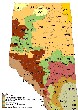
Figure 1. Location of 42 benchmark sites across Alberta.
This report examines the following aspects of the first five years of data from the Soil Quality Benchmark Program:
| 1. | Variation in soil properties from year to year within sites to estimate when significant change could be determined. |
| 2. | Differences among ecoregions [Peace Lowland (PL), Mixed Boreal Uplands (MB), Boreal Transition (BT), Aspen Parkland (AP), Moist Mixed Grassland (MM), Fescue Grasslands (FG), and Mixed Grassland (MG)]. |
| 3. | Differences among slope positions (upper, mid and lower slopes were sampled at each of the 42 benchmark sites). |
| 4. | Effects of management (cropping systems or tillage). |
Objectives
The objectives of the soil-quality monitoring program as stated by Leskiw et al. (2000), were as follows:
"The soil quality monitoring program is designed to determine the state of soil quality across Alberta and to evaluate the change in soil quality under the influence of various management practices. The objectives of using benchmark sites are to: assess wind and water erosion; determine landscape and soil quality variables; and to monitor changes in soil quality over time".
This report examines the data from the first five years of the study. The objectives were to:
| 1. | Review the database (1998 to 2002) for data integrity; |
| 2. | Conduct various statistical analyses to examine variation and trends; |
| 3. | Examine yearly variation and trends of various soil properties with respect to ecoregion, site characteristics, landform and management practices. |
Methods
Data were examined from soil samples (0-15 cm and 15-30 cm) taken for fertility analysis. Soil samples were taken in the fall, after harvest, but before freeze-up and prior to fall fertilization. Composite samples of five to ten cores were collected within a radius of two meters from the central marker at each of the landscape positions (upper, mid and lower slope positions). The soil analyses included pH in water (pHw), pH in CaCl2 (pHc), EC, free lime (CaCO3), NO3-N, NH4-N, P, K, S, organic matter (OM), hot KCl extractable NH4-N, bulk density (BD), light fraction mass (LF_mass), light fraction carbon (LFC) and light fraction nitrogen (LFN).
Descriptive statistical procedures [mean, max, min, standard deviation (SD) and coefficient of variation (CV)] were used for initial examination of the data and to evaluate yearly variation in soil properties at each sampling location (upper, mid and lower slope positions at the 42 benchmark sites). It was noted that the CVs of soil properties measured over the five-year period were much higher at some sites than at others. Therefore, the variability of sites and sampling locations was classified based on the CVs of relatively stable soil properties (pH, EC, P, K, and LF_mass).
Analysis of variance (General Linear Model procedure in SAS) was used to examine differences among ecoregions and slope positions. Years were treated as replicates and Student-Newman-Keuls was used for mean comparisons when the F test was significant (p < 0.05).
Main Findings
Descriptive statistics
Appendices 1 and 2 provide all of the data for the fourteen soil properties analyzed. Mean, max, min, SD and CV (%) values are shown for each ecoregion and the CV for each sampling location (site x 3 slope positions) over the five-year period.
Effect of ecoregions, slope positions and management practices
Differences among ecoregions
There were relatively few significant differences in soil properties among the ecoregions, indicating that differences within ecoregions were often as large as between ecoregions (Table 1). Soil properties were averaged across all three landscape positions and corresponding sites for each ecoregion. There were no significant differences in pHw, pHc, EC, NH4-N, NO3-N, P, S, BD, and CaCO3 between any of the ecoregions. OM, LF_mass, Hot KCl NH4-N and CEC were lower in the MG Ecoregion than in the other ecoregions, but there were no differences among the other ecoregions. The low values for LF_mass, OM and CEC, and the high CaCO3 value are characteristic of the MG Ecoregion (Brown Soil Zone). The relatively high BD in the MG Ecoregion would also be expected because of the low soil OM.
Other differences among ecoregions include:
| 1. | Extractable K was lowest in the BT Ecoregion. It was significantly lower than in the MM, FG, and MG Ecoregions. This trend is consistent with summaries of routine soil test data for fertility evaluation. |
| 2. | OM was lower in the MG Ecoregion than in all other ecoregions, except MM. |
| 3. | LF_mass was highest in the FG Ecoregion and lowest in the MM Ecoregion. |
| 4. | Hot KCl NH4-N is significantly lower in the MG than in the AP Ecoregion. |
| 5. | Clay (%) was highest in the PL Ecoregion, but only significantly different from the MM Ecoregion. |
| 6. | The PL Ecoregion had the highest CEC (significantly higher than MG). This is consistent with the high clay content of the sites in the PL Ecoregion. |
The low BD, and high LF_mass and OM, in the MB Ecoregion, are uncharacteristic. The MB Ecoregion is represented by only one site. The upper slope position at this site has many values that are very atypical (the upper slope position is likely on an area where large amounts of straw or brush piles were burned). The MB site was removed from the dataset (because of high variability and having only one site in its respective ecoregion) before statistical analyses on ecoregions was determined. However, the descriptive analyses for the MB Ecoregion were still documented.
Differences among slope positions
Analysis Of Variance (ANOVA) was used to identify differences in the five-year mean values for upper, mid and lower slope sampling positions. Significant differences among slope positions were observed for pHw, pHc, NO3-N, P, K, S, OM, Hot KCl NH4-N, BD and clay (Table 2). In this case, soil properties were averaged across all 42 sites. Generally, the lower slope position had significantly higher values of NO3-N, P, K, S, OM, and Hot KCl NH4-N when compared to the mid or upper slope positions. In contrast, BD values for the lower slope position were lower than those of the upper or mid slope position. Upper slope positions had significantly higher values of pHw and pHc than both the mid and lower slope positions. There were no significant differences among the three slope positions for EC, NH4-N, LF_mass, CEC or CaCO3.
In contrast to ecoregions where relatively large differences were not significant, relatively small differences among slope positions were often significant. For example, the mean pH of sites in the MG Ecoregion (7.3) was not significantly different from the MM Ecoregion (6.3), but the mean pH of upper slopes (6.7) was significantly higher than for the mid and lower slopes (6.5) [Tables 1 and 2]. The lack of significant differences in soil properties between ecoregions is in part a result of large variations in properties within ecoregions but it should also be noted that the statistical power for testing differences between slope positions is greater than between ecoregions. The magnitude of the difference required for statistical significance between ecoregions compared to slope positions is illustrated in Figures 2 to 5.
Effect of management
There were no significant effects of cropping system or tillage on the soil properties measured except that LF_mass was sometimes higher on tilled or annual cropping sites than on minimum or no-till sites or sites that included forages. This is opposite to what would be expected. The nature of this study does not provide for the comparison of management practices that are adjacent under the same soil and environmental conditions. Factors other than tillage, such as cropping systems and climate, can affect LF_mass (see comments under recommendations).
Variation in soil properties
Variability for soil properties at each of the sites within ecoregions and within slope positions was determined across all five years. As well, variability for each site within separate sampling years was determined across all ecoregions and slope positions. The mean coefficients of variation (CV) for NH4-N, NO3-N, S and LF_mass were higher than for pH, EC, P, K, OM, LFC, LFN, and BD (Table 3). The high variability of NH4, NO3, and SO4 would be expected, since they can change rapidly due to mineralization, nitrification and crop removal. However, the high CV for LF_mass (45.6%) would not be expected. LF_mass consists of rapidly cycling organic matter derived from recent additions of crop residue, which may not be evenly distributed. Therefore, this could lead to large sampling errors. LF_mass is also affected by cropping systems, tillage and climate conditions but this should not result in large variations from year to year within a sampling location.
Table 1.� Effect of ecoregions on some soil properties1 (0-15 cm) averaged across all landscape positions for the past five years.
Eco-
region | No. of
sites | pHw | pHc | EC
(dS/m) | NH4-N
(mg/kg) | NO3-N
(mg/kg) | P
(mg/kg) | K
(mg/kg) | S
(mg/kg) | OM
(%) | LF_mass
(mgLFC/g) | Hot KCl NH4-N
(mg/kg) | BD
(g/cm3) | Clay
(%) | CEC
(meq/100g) | CaCO3
(%) |
PL | 9 | 6.6 | 5.8 | 0.58 | 1.48 | 15.4 | 23 | 256bc* | 16.5 | 6.9a | 7.0ab | 34.9ab | 1.29 | 36a | 28.9a | 0.74 |
MB | 1 | 6.7 | 6.2 | 0.68 | 1.88 | 24.0 | 39 | 254 | 11.1 | 11.1 | 18.6 | 47.1 | 1.06 | 16 | 20.6 | 1.53 |
BT | 8 | 6.4 | 5.7 | 0.45 | 1.84 | 7.7 | 17 | 188c | 11.0 | 5.7a | 7.2ab | 32.4ab | 1.33 | 26ab | 24.1ab | 0.77 |
AP | 9 | 6.4 | 5.7 | 0.52 | 3.89 | 13.5 | 22 | 280bc | 17.8 | 6.7a | 7.4ab | 39.6a | 1.31 | 21ab | 24.6ab | 0.72 |
MM | 5 | 6.3 | 5.6 | 0.49 | 1.68 | 13.2 | 26 | 348b | 12.7 | 4.4ab | 7.2ab | 22.1bc | 1.33 | 18b | 18.0ab | 0.70 |
FG | 2 | 6.3 | 5.6 | 0.34 | 1.86 | 10.1 | 23 | 497a | 6.0 | 6.5a | 8.8a | 32.9ab | 1.29 | 29ab | 26.1ab | 0.70 |
MG | 8 | 7.3 | 6.7 | 0.58 | 1.50 | 8.8 | 17 | 326b | 12.3 | 2.4b | 3.7b | 15.6bc | 1.47 | 24ab | 15.7b | 1.85 |
1 pHw, pHc, EC, NH4-N, NO3-N, P, K, S, OM, LF_mass, Hot KCl NH4-N, and BD sampled every year; clay, CEC, CaCO3 sampled only in the establishment year.
*ecoregion means followed by the same letter are not significantly difference at p < 0.05.
Table 2.� Effect of slope position on some soil properties1 (0-15 cm) averaged across all sites for the past five years.
Slope
Position | pHw | pHc | EC
(dS/m) | NH4-N
(mg/kg) | NO3-N
(mg/kg) | P
(mg/kg) | K
(mg/kg) | S
(mg/kg) | OM
(%) | LF_mass
(mgLFC/g) | Hot KCl NH4-N
(mg/kg) | BD
(g/cm3) | Clay
(%) | CEC
(meq/100g) | CaCO3
(%) |
| Upper | 6.7a* | 6.0a | 0.55 | 2.28 | 10.5b | 20b | 264b | 12.0b | 4.6c | 6.5 | 26.0c | 1.38a | 27a | 23 | 1.10 |
| Mid | 6.5b | 5.8b | 0.48 | 2.29 | 11.6ab | 18b | 259b | 10.1b | 5.2b | 6.6 | 30.4b | 1.36a | 25b | 23 | 0.83 |
| Lower | 6.5b | 5.8b | 0.53 | 1.77 | 13.7a | 26a | 328a | 19.3a | 6.9a | 7.6 | 34.9a | 1.26b | 26ab | 25 | 0.88 |
1 pHw, pHc, EC, NH4-N, NO3-N, P, K, S, OM, LF_mass, Hot KCl NH4-N, and BD sampled every year; clay, CEC, CaCO3 sampled only in the establishment year.
* slope position means followed by the same letter are not significantly different at p < 0.05
Some of the variation in LF_mass may also be a result of measurement error. The determination of LF_mass tends to be subject to greater laboratory error than is the case with other soil properties (Solberg, E., personal communication).
The variability of NO3-N and LF_mass within each sampling year (Table 5) was lower than in the five-year data (Table 3). For example, the mean CV for NO3-N was 66.6% for ecoregions, but only 41% within separate sampling years. This suggests that variability from year to year may reflect management and climate conditions as well as sampling error.
In a study in Wisconsin, Kucharik et al. (2003), using 14 paired sites (composite samples of 15 core from paired transects on cropped land and adjacent land in the Conservation Reserve Program for >8 years), found that C and N storage rates were highly variable among sites (CVs > 20%). Using a minimum detectable difference method (MDD), 40 to 65 paired sites and sampling in 5 cm increments near the surface were needed to achieve an 80% confidence level (a = 0.05; B = 0.20) in C and N sequestration rates. Given these results and the relatively high CVs for OM and LF_mass in this study, the sampling intensity and methodology should be reviewed. The current methodology and analyses detected relatively small differences among slope positions but not among Ecoregions or management systems.
Table 3. Mean coefficient of variation (CV %) within ecoregions for 14 soil properties over a five- year period.
| Eco-region | pHw | pHc | EC | NH4-N | NO3-N | P | K | S | OM | LFC | | LFN | Hot KCl NH4-N | BD |
| PL | 3.1 | 3.2 | 31.4 | 79.7 | 59.2 | 16.6 | 20.0 | 49.6 | 6.1 | 16.1 | 54.9 | 16.0 | 23.1 | 9.7 |
| MB | 5.6 | 7.7 | 39.9 | 54.8 | 108.0 | 43.1 | 41.7 | 37.0 | 24.6 | 11.3 | 66.2 | 11.2 | 31.9 | 21.0 |
| BT | 3.1 | 4.5 | 33.3 | 65.9 | 70.0 | 21.0 | 21.6 | 55.4 | 15.1 | 15.7 | 36.7 | 16.6 | 28.5 | 10.0 |
| AP | 4.2 | 4.1 | 41.3 | 93.9 | 66.5 | 28.1 | 29.2 | 59.2 | 8.8 | 16.3 | 38.5 | 12.5 | 33.7 | 9.1 |
| MM | 4.5 | 4.3 | 33.1 | 79.7 | 67.8 | 29.5 | 20.2 | 56.9 | 10.9 | 18.3 | 48.7 | 17.8 | 24.6 | 12.2 |
| FG | 4.9 | 6.5 | 39.5 | 86.2 | 75.0 | 33.0 | 25.3 | 54.1 | 7.7 | 29.5 | 79.9 | 25.3 | 21.2 | 11.4 |
| MG | 3.5 | 5.8 | 28.8 | 94.9 | 64.0 | 30.5 | 25.8 | 49.2 | 11.1 | 28.1 | 38.9 | 26.5 | 28.2 | 9.7 |
| Mean | 3.7 | 4.0 | 34.2 | 82.7 | 66.6 | 25.5 | 24.4 | 53.5 | 10.4 | 19.1 | 45.6 | 17.9 | 27.6 | 10.3 |
Effect of ecoregion on year-to-year variation of relatively stable soil properties
Variation from year to year in the more stable soil properties (pHw, EC, P, K and LF_mass) was greater in some ecoregions than in others (Table 4). Variability was lowest in the PL and BT Ecoregions and highest in the FG, and MB Ecoregions (note: there were only two sites in the FG Ecoregion and one site in the MB Ecoregion). While the variation among years for the more stable properties was lower than for variable properties such as NO3 and NH4, it was still relatively high at many sites, indicating that large changes in these properties would have to occur before significant trends could be detected.
Effect of slope position and year on variation of relatively stable soil properties
The effect of slope position and year on variability of seven soil properties is summarized in Tables 4 and 5. The CVs of the three slope positions and years were similar for the seven parameters shown in Table 4. Also, the CVs were similar for each of the five years (Table 5), indicating that the inherent variability of these parameters was not influenced by year.
Table 4. Mean coefficient of variation (CV %) of slope positions for several soil properties (0-15 cm ) over a five year period.
| Slope Position | No. of Sites | pHw | EC | P | K | LF_mass | NO3-N | BD |
| Upper | 42 | 3.8 | 36 | 28 | 25 | 45 | 63 | 9.2 |
| Mid | 42 | 3.4 | 35 | 25 | 23 | 45 | 66 | 9.6 |
| Lower | 42 | 4.0 | 32 | 24 | 25 | 46 | 71 | 12.1 |
Table 5. Mean coefficient of variation (CV %) for years (0-15 cm).
| Year | No. of Sites | pHw | EC | P | K | LF_mass | NO3-N | BD |
| 1998 | 37 | 6.2 | 29 | 43 | 33 | 37 | 41 | 8.3 |
| 1999 | 41 | 5.3 | 35 | 42 | 30 | 32 | 45 | 8.5 |
| 2000 | 42 | 5.5 | 30 | 37 | 26 | 31 | 40 | 9.3 |
| 2001 | 42 | 4.7 | 29 | 35 | 23 | 28 | 40 | 8.6 |
| 2002 | 42 | 5.6 | 28 | 36 | 27 | 39 | 39 | 9.6 |
Variation from year-to-year within sampling location (slope positions within sites)
Variability of each sampling location (42 sites x 3 slope positions = 126 locations) was assessed using the CVs for pHw, EC, P, K and LF_mass. These properties were considered to be inherently less variable from year to year than properties such as NO3-N, NH4-N and S. [Note: Soil organic matter (OM) is also a relatively stable soil parameter as indicated by the low CV (Table 3). However, it was not included as a parameter in classifying the variability of the sites because the five-year data was not available when this analysis was conducted]. BD was not used because it was not analysed each year at all sites. A sampling location was classified as moderately variable when 3 of the 5 properties (pHw, EC, P, K, and LF_mass) were above a threshold CV value and highly variable when 4 or 5 of the properties were above a threshold value. The threshold CV values used were: pHw > 4; EC > 40; P > 25; K > 25; LF_mass >25.
The number and percentage of locations classified as moderately or highly variable are shown in Table 6. The lowest percentage of variable sampling locations occurred in the PL and BT Ecoregions. The highest percentage occurred in the AP and MM Ecoregions. The MB and FG Ecoregions also had high percentages of variable locations, but they were represented by only one and two sites, respectively. Overall, 23 of 126 locations (18%) were classified as highly variable and 38 of 126 (29%) were classified as moderately variable.
Table 6. Number and percentage of variable sampling locations within each ecoregion
| Ecoregion | No. of
Locations | Moderately Variable (%) | Highly Variable (%) | Mod. & Highly Variable (%) |
| PL | 27* | 3/27� (11.1) | 1/27� (3.7) | (14.8) |
| MB | 3 | 0/3���� (0) | 2/3�� (67) | (67) |
| BT | 24 | 8/24� (33) | 1/24� (4.2) | (37) |
| AP | 27 | 13/27 (48) | 6/27� (22) | (70) |
| MM | 15 | 5/15� (33) | 6/15� (40) | (73) |
| FG | 6 | 2/6��� (33) | 2/6�� (33) | (66) |
| MG | 24 | 5/24� (21) | 5/24� (21) | (48) |
* no. of sites within ecoregion x 3 slope positions.
Variation within benchmark sites
The variability of each site was also assessed using the variability of the 3 sampling locations upper (U), mid (M) and lower (L) slopes. Sites with 2 of the slope positions with a score of 3 or more were classified as moderately variable (3 or more of the 5 variable above the threshold value 3). Sites were classified as highly variable when all 3 slope positions had a score of 3 or more.
- PL - only one site was moderately variable (599 - M = 3, L = 4).
- MB- site 615 was moderately variable (U = 4, L = 4).
- Note: there is only one site in the MB Ecoregion and some of the properties in the U and L slope positions are extremely variable
- BT - Site 678 was moderately variable (U = 3, L = 3)
- Site 680 was highly variable (U = 3, M = 3, L = 3)
- Note: 692 (U= 4)
- AP - 727 moderately variable (U = 3, M = 3)
- 743 moderately variable (M = 3, L = 5)
- 744 moderately variable (U = 4, M = 3)
- 730 highly variable (U = 3, M = 4, L = 3)
- 739 highly variable (U = 3, M = 3, L = 3)
- 740 highly variable (U = 3, M = 4, L = 4)
- 746 highly variable (U = 3, M = 3, L = 3)
- Note: 692 U = 4, 728 L = 4, 738 L = 4
- MM - 769 moderately variable (U = 4, M = 3)
- 786 moderately variable (U = 4, L = 3)
- 781 highly variable (U = 4, M = 5, L = 3)
- Note: 791 (U = 4)
- FG - 800 moderately variable (U = 3, M = 4)
-798 Highly variable (U = 4, M = 5, L = 3)
- MG - 806 moderately variable (M = 4, L = 4)
- 2828 moderately variable (U = 3, L = 3)
- 804 highly variable (U = 3, M = 4, L = 4)
From the above, 8 sites (19%) were highly variable and 11 (26%) moderately variable. The site in the MB Ecoregion should also be considered to be highly variable because some properties at the upper and lower slope positions have been extremely variable from year to year. Four of the highly variable sites were in the AP Ecoregion (4 of 9); one in BT (1 of 8); one in MM (1 of 5); one in FG (1 of 2); and one in MG (1 of 8).
Notes on variability of specific sampling locations
The following sampling locations were noted because a high CV resulted mainly from one 'outlier' value or in the case of pH, inconsistencies between pHw and pHc values. Some of these may be analysis or recording errors and should be reanalysed.
| Site No. | Slope Position | Comments |
| 586 | L | 1999 - pHw is high (rerun) |
| 591 | U | 2002 – pHw, pHc and EC are high |
| 595 | U | 2000 – P high (rerun) |
| 599 | U
U,M,L | 1999 – EC is very high; likely a recording error
2002 – K is high |
| 680 | L | 2001 – pHw (7.2) and pHc (5.6) (rerun) |
| 687 | U | 1998 – pHw (6.4) and pHc (5.2) (rerun);
2001 and 2002 – high P |
| 728 | L | 2001 – pHw and pHc both high |
| 738 | U,M,L | 1998 – pHw is high and pHc is low |
| 740 | L | 2002 – P and K very high but not on U and M (rerun) |
| 746 | U,M,L | 2002 – high P |
| 781 | L
U, M | 1998 – pHw is high and pHc low (rerun)
1999 – P is low (rerun) |
| 804 | M,L | 2000 – pH is high (rerun) |
| 809 | L | 1999 – pHc (7.1) is higher than pHw (6.9) (rerun) |
| 2828 | U,M,L | Note – only 3 years of data (2000, 2001 and 2002) |
Summary
The inherent spatial variability of soil properties (both within defined soil/landforms as seen in variation among individual cores or composites of a small number of cores; or larger scale variability across soil/landforms) creates difficulties in identifying change. If variation among samples taken from the same sampling location is high, then large changes in soil properties must occur to identify a significant trend. Morton et al. (2000) found that much of the total field variation in pH, K, P, S and C occurred within the first meter. This indicates that even with site-specific sampling (in this study, the sampling sites have a 1 m radius), 20 or more cores may be required to reduce sampling error to an acceptable level.
In field experiments where differences in management practices are imposed in a randomized and replicated pattern, a minimum of five to 10 years is often required to identify significant changes in soil properties. Field plots are designed to eliminate or minimize soil variability in order to isolate treatment effects. Conversely, the extensive nature and design of the Soil Quality Benchmark Study provides data over a wide range of soil properties, climate and management, but the lack of replicate sampling (replicates within the same year) will result in a longer time frame to detect significant changes in soil properties. On the other hand, the diversity encompassed in the design provides a database useful for model validation and for scaling up agronomic and soil quality information to a provincial scale.
The data from the 42 AESA Benchmark Sites have revealed differences in several parameters within different ecoregions and within slope positions. Within ecoregions, differences in OM, LF_mass, Hot KCl NH4-N, K, Clay and CEC were observed. Within landscape positions, differences in pHw, pHc, NO3-N, P, K, S, OM, LF_mass, Hot KCl NH4-N, BD and clay content were observed. The importance of landscape sampling can't be emphasized enough since average values from composite samples taken across slope positions would not have demonstrated significant differences for several soil parameters.
Recommendations
| 1. | Review sampling methodology/protocol and intensity:
- Compare current and more intensive sampling on sites that have been identified as variable (high CVs) and uniform (low CVs).
- Consider sampling depth intervals of 5 cm for LF_mass, OM and BD (LF_mass and OM values should be expressed on an equivalent mass basis).
|
| 2. | Conduct repeat analysis for LF_mass on some samples to determine confidence limits of this method.
. |
| 3. | The author and Karen Cannon consulted with biostatisticians regarding the sampling protocol and the variability of the data from some of the sites. The main questions were:
- Is sampling every year required?
- Are replicate samples within years required?
- Would trend analysis be useful at this point in the study?
The biostatisticians generally indicated that for trend analysis, sampling every year would be better than at intervals of 2 or 3 years with replicate samples within years. (Sampling every year, with replicates within years, would be ideal, but it is considered too costly). Initial attempts at trend analysis could be useful with 6 to 7 years of data.
. |
4.
| This initial analysis of the data made limited use of the management information being collected. The management information could be utilized more effectively in the future if site information was classified on the basis of both the type (tillage system, crop rotation) and level of management [input level and effectiveness of the overall management (productivity index)]. |
References
Cannon, K.R. 2002. Alberta Benchmark Site Selection and Sampling Protocols. Prepared for the AESA Soil Quality Resource Monitoring Program. Conservation and Development Branch. Alberta Agriculture, Food and Rural Development. Edmonton, Alberta. 43 pp.
Cannon, K. and Leskiw, L. 1999. Soil Quality Benchmarks in Alberta. In: Proceedings of 36th Annual Alberta Soil Science Workshop, February 16-18, 1999, Calgary, Alberta. pp. 181-183.
Garten, C.T. and Wullschleger, S.D. 1999. Soil carbon inventories under a bioenergy crop (Switchgrass): measurement limitations. Journal of Environmental Quality 28: 1359-1365.
Janzen, H.H., Campbell, C.A., Gregorich, E.G., and Ellert, B.H. 1998. Soil Carbon Dynamics in Canadian Agroecosystems. In: Soil Processes and the Carbon Cycle (Advances in Soil Science). Lal, R, Kimble, J.M., Follett, R.F. and Stewart, B.A. (eds). Chapter 5. CRC Press LLC, Boca Raton, Florida, USA.
Kucharik, C.J., Roth, J.A. and Nabielski, R.T. 2003. Statistical assessment of a paired-site approach for verification of carbon and nitrogen sequestration on Wisconsin Conservation Reserve Program land. Journal of Soil and Water Conservation. 58(1): 58-65.
Leskiw, L.A. Yarmuch, M.S., Waterman, B.A., and Sansom, J.J. 2000. Baseline Soil Physical and Chemical Properties of Forty-three Soil Quality Benchmark Sites in Alberta. Prepared for the AESA Soil Quality Resource Monitoring Program. Conservation and Development Branch. Alberta Agriculture, Food and Rural Development. Edmonton, Alberta. 175 pp.
Morton, J.D., Baird, D.B. and Manning, M.J. 2000. A soil sampling protocol to minimize the spatial variability in soil test values in New Zealand hill country. New Zealand Journal of Agricultural Research. 43: 367 - 375.
Solberg, Elston. 2004. Personal communication. Agri-Knowledge Division Manager, Sun Mountain Agronomy.
Acknowledgements
The author would like to acknowledge the help of several individuals and groups in the development of the AESA Soil Quality Benchmark Database and the preparation of this report. I would like to thank Karen Cannon for statistical analysis and consultation throughout the preparation of the report; Jody Winder for help with data validation, tables, appendices and sample preparation; the AESA Regional Conservation Staff for soil and crop sampling; Norwest Labs for soil and plant analysis; Tom Goddard for review and suggestions; and Deb Sutton for final manuscript preparation.
D. Penney
Prepared for:
Alberta Environmentally Sustainable Agriculture (AESA)
Soil Quality Monitoring Program
Alberta Agriculture, Food and Rural Development
Conservation and Development Branch
#206, 7000 - 113 Street
Edmonton, Alberta
Canada T6H 5T6 |
|