| | Light | Temperature management | Management of the relative humidity using vapour pressure deficits | Carbon dioxide supplementation | Air pollution in the greenhouse | Growing media | Management of irrigation and fertilizer feed | Rules for mixing fertilizers | Application of fertilizer and water
This section looks at how the tools that growers have at their disposal to control the environment, are manipulated with respect to the important environmental influences on plant growth and development, for the actual optimization of the greenhouse environment. As stated in "Concepts Involved in the Optimization of the Greenhouse Environment for Crop Production," the primary goal of optimization of the greenhouse environment is to maximize the photosynthetic process in the crop. The strategy used to maximize photosynthesis is through the management of transpiration. Therefore, on-going modifications are made to the greenhouse environment to manage the transpiration of the crop to match the maximum rate of photosynthesis.
Growth can be defined as an increase in biomass (Papadopoulos and Pararajasingham 1997). The increase in size of a plant or other organism can also be considered as the fundamental definition of growth (Salisbury and Ross 1978). The growth of plants is associated with changes in the numbers of plant organs occurring through the initiation of new leaves, stems and fruit, abortion of leaves and fruit, and physiological development of numbers from one age class to the next (Jones et al 1989). Managing growth and development of an entire crop for maximum production involves the manipulation of temperature and humidity to obtain not only the maximum rate of photosynthesis under the given light conditions, but also the optimum balance of vegetative and generative growth of plants for sustained production and high yields (Portree 1996). This implies that growers can direct the results of photosynthesis, the production of assimilates, sugars and starches, towards both vegetative and generative in a balance.
Generative growth is the growth associated with fruit production. For maximum fruit production to occur, the plant has to be provided both with the appropriate cues to trigger the setting of fruit and the cues to maintain adequate levels of stem and leaf development. The balance is achieved when the assimilates from photosynthesis are directed towards maintaining the production of the new leaves and stems required to support the continued production of fruit. The appropriate cues are provided through the manipulation of the environment, and are subject to change depending on the behavior of the crop. Careful attention must be paid to the signals given by the plant, the indicators of which direction the plant is primarily headed, vegetative or generative, and how corrective action is applied through further manipulation of the environment to maintain high production.
Light
Light limits the photosynthetic productivity of all crops (Wilson et al 1992) and is the most important variable affecting productivity in the greenhouse (Wilson et al 1992, Papadopoulos and Pararajasingham 1997). The transpiration rate of any greenhouse crop is the function of three variables; ambient temperature, humidity and light (Stanghellini and Van Meurs 1992, Van Meurs and Stanghellini 1992). Of these three, it is light which is usually out of our control as it is received from the sun (Stanghellini and Van Meurs 1992, Van Meurs and Stanghellini 1992). Supplementary lighting does offer opportunity to increase yield during low light periods, but is generally considered commercially unprofitable (Warren et al 1992, Papadopoulos and Pararajasingham 1997). The other means for manipulating light are limited to screening or shading (Stanghellini and Van Meurs 1992) and are employed when light intensities are too high. However, there are also general strategies to help maximize the crop's access to the available light in the greenhouse.
Properties of light and its measurement
In order to understand how to control the environment to make the maximum use of the available light in the greenhouse, it is important to know about the properties of light and how light is measured. Considerable confusion has existed regarding the measurement of light (LI-COR Inc.), however it is worthwhile for growers to approach the subject.
Light has both wave properties and properties of particles or photons (Tilley 1979). Depending on how light is considered, the measurement of light can reflect either its wave or particle properties. Different companies provide a number of different types of light sensors for use with computerized environmental control systems. As long as the sensors measure the light available to plants, for practical purposes it is not as important how light is measured, as it is for growers to be able to relate these measurements to how the crop is performing.
Light is a form of radiation produced by the sun, electromagnetic radiation. A narrow range of this electromagnetic radiation falls within the range of 400 to 700 nanometers (nm) of wavelength. One nanometer being equal to 0.000000001 meters. The portion of the electromagnetic spectrum which falls between 400 to 700 nm is referred to as the spectrum of visible light, this is essentially the range of the electromagnetic spectrum that can be seen. Plants respond to light in the visible spectrum and use this light to drive photosynthesis.
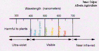
Figure 14. The visible spectrum.
Photosynthetically Active Radiation (PAR) is defined as radiation in the 400 to 700 nm waveband. PAR is the general term which covers both photon terms and energy terms ( LI-COR Inc.). The rate of flow of radiant (light) energy in the form of an electromagnetic wave is called the radiant flux, and the unit used to measure this is the Watt (W). The units of Watts per square meter (W/m�) are used by some light meters and is an example of an "instantaneous" measurement of PAR (LI-COR Inc.). Other meters commonly seen in greenhouses take "integrated" measurements reporting in units of joules per square centimeter (j/cm�) (LI-COR Inc.). Although the units seem fairly similar, there is no direct conversion between the two. Photosynthetic Photon Flux Density (PPFD) is another term associated with PAR, but refers to the measurement of light in terms of photons or particles. It is also sometimes referred to as Quantum Flux Density (LI-COR Inc.). Photosynthetic Photon Flux Density is defined as the number of photons in the 400 - 700 nm waveband reaching a unit surface per unit of time (LI-COR Inc.). The units of PPFD are micromoles per second per square meter (micromol/m�).
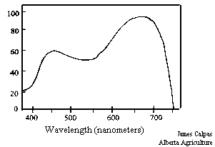
Figure 15. The photosynthetic action spectrum.
As the scientific community begins to agree on how best to measure light there may be more standardization in light sensors and the units used to describe the light radiation reaching a unit area. Greenhouse growers will still be left with the task of making day-to-day meaning of the light readings with respect to control of the overall environment. Generally speaking, the more intense the light, the higher the rate of photosynthesis and transpiration (increased humidity), as well as solar heat gain in the greenhouse. Of these, it is heat gain which usually calls for modification of the environment as temperatures rise on the high end of the optimum range for photosynthesis, and ventilation and cooling begins. Plants also require more water under increasing light levels.
The light use efficiency of plants
Plants use the light in the 400 to 700 nm range for photosynthesis, but they make better use of some wavelengths than others. Figure 15 presents the photosynthetic action spectrum of plants, the relative rate of photosynthesis of plants over the range of PAR, photosynthetically available light. All plants show a peak of light use in the red region, approximately 650 nm and a smaller peak in the blue region at approximately 450 nm (Salisbury and Ross 1978). Plants are relatively inefficient at using light and are only able to use about a maximum of 22% of the light absorbed in the 400 to 700 nm region (Salisbury and Ross 1978). Light use efficiency by plants depends not only on the photosynthetic efficiency of plants, but also on the efficiency of the interception of light (Wilson et al 1992).
Maximizing the crop's access to available light
The high cost of greenhouse production requires growers to maximize the use of light falling on the greenhouse area ( Wilson et al 1992). Before the crops are able to use the light, it first has to pass through the greenhouse covering, which does not transmit light perfectly. The greenhouse intercepts a percentage of light falling on it allowing a maximum of 80% of the light to reach the crop at around noon, with an overall average of 68% over the day (Wilson et al 1992). However, the greenhouse covering also partially diffuses or scatters the light coming into the greenhouse so that it is not all moving in one direction (Wilson et al 1992). The implication of this is scattered light tends to reach more leaves in the canopy than directional light which throws more shadows.
It is important that the crop be orientated in such a way that the light transmitted through the structure is optimized to allow for efficient distribution to the canopy. Greenhouse vegetable crops have a vertical structure in the greenhouse, so light filters down through "layers" of leaves before a smaller percentage actually reaches the floor. Leaf area index (LAI) is widely used to indicate the ratio of the area of leaves over the area of ground which the leaves cover (Salisbury and Ross 1978). Leaf area indexes of up to 8 are common for many mature crop communities, depending on species and planting density (Salisbury and Ross 1978). Mature canopies of greenhouse sweet peppers have a relatively high leaf area index of approximately 6.3 when compared to greenhouse cucumbers and tomatoes at 3.4 to 2.3 respectively (Hand et al 1993).
The optimum leaf area index varies with the amount of sunlight reaching the crop. Under full sun, the optimum LAI is 7, at 60% of full sun the optimum is 5, at 23% full sunlight, the optimum is only 1.5 (Salisbury and Ross 1978). This point has application to a growing and developing crop. In Alberta, vegetable crops are seeded in November to December, the low light period of the year. Young crops have lower leaf area indexes which increase as the crop ages. Under this crop cycle, the plants are growing and increasing their LAI as the light conditions improve. Crop productivity increases with LAI up to a certain point because of more efficient light interception, as LAI increases beyond this point no further efficiency increases are realized, and in some cases decreases occur (Salisbury and Ross 1978).
There is also a suggestion that an efficient crop canopy must allow some penetration of PAR below the uppermost leaves, and the sharing of light by many leaves is a prerequisite of high productivity (Papadopoulos and Pararajasingham 1997). Leaves can be divided into two groups; sun leaves that intercept direct radiation and shade leaves, that receive scattered radiation (Wilson and Loomis 1967, Papadopoulos and Pararajasingham 1997). The structures of these leaves are distinctly different (Wilson and Loomis 1967).
The major greenhouse vegetable crops (tomatoes, cucumbers and peppers) are arranged in either single or double rows (Wilson et al 1992, Hand et al 1993). This arrangement of the plants and subsequent canopy represents an effective compromise between accessibility to work the crop, and light interception by the crop (Hand et al 1993). For a greenhouse pepper crop, this canopy provides for light interception exceeding 90% under overcast skies and 94% for much of the day under clear skies (Hand et al 1993). There is a dramatic decrease in interception that occurs around noon, and lasts for about an hour when the sun aligns along the axis of north - south aligned crop rows. Interception falls to 50% at the gap centers where the remaining light reaches the ground, and the overall interception of the canopy drops to 80% (Hand et al 1993).
The strategies to reduce this light loss would be to align the rows east-west instead of north-south, reduced light interception occurring when the sun aligns with the rows would take place early and late in the day when the light intensities are already quite low (Hand et al 1993). The use of white plastic ground cover can reflect back light that has penetrated the canopy and can result in an overall increase of 9% over crops without white plastic ground cover (Wilson et al 1992, Hand et al 1993).
The effect of row orientation varies with time of the day, season, latitude and canopy geometry (Papadopoulos and Pararajasingham 1997). It has been demonstrated that at 34� latitude, north-south orientated rows of tall crops, such as tomatoes, cucumbers and peppers, intercepted more radiation over the growing season than those orientated east-west (Papadopoulos and Pararajasingham 1997). This finding was the opposite for crops grown at 51.3� latitude (Papadopoulos and Pararajasingham 1997). The majority of greenhouse vegetable crop production in Alberta occurs between 50� (Redcliff) and 53� (Edmonton) North. This would suggest that the optimum row alignment of tall crops for maximum light interception over the entire season, would be east-west. However, in Alberta, high yielding greenhouse vegetable crops are grown in greenhouses with north-south aligned rows as well as in greenhouses with east-west aligned rows.
Alberta is known for its sunshine, and the sun is not usually limiting during the summer. In fact, many vegetable growers apply whitewash shading to the greenhouses during the high light period of the year because the light intensity and associated solar heat gain can be too high for optimal crop performance. The strategies for increasing light interception by the canopy should focus specifically on the times in year when light is limiting, for Alberta, this is early spring and late fall. When light is limiting, a linear function exists between light reduction and decreased growth, with a 1% increase in growth occurring with a 1% increase in light (De Koning 1989, Wilson et al 1992) under light levels up to 200 W/m�.
When light levels are limiting, supplementary artificial lighting will increase plant growth and yield (Papadopoulos and Pararajasingham 1997). The use of supplemental lighting has its limits as well. Using supplemental lighting to increase the photoperiod to 16 and 20 hours increased the yield of pepper plants while continuous light decreased yields compared to the 20 hour photoperiod (Demers and Gosselin 1998). The economics of artificial light supplementation generally do not warrant the use of supplementary light on a greenhouse vegetable crop in full production. However, supplementary lighting of seedling vegetable plants prior to transplanting into the production greenhouse is recommended for those growers growing their own plants from seed.
Light is generally limiting in Alberta when greenhouse vegetable seedlings are started in November to December. Using supplemental lighting for seedling transplant production when natural light is limiting resulted in increased weight of tomato and pepper transplants grown under supplemental light compared to control transplants grown under natural light (Demers et al 1991, Fierro et al 1994). Young plants exposed to supplemental light also were ready for transplanting 1 to 2 weeks earlier than plants grown under natural light (Demers et al 1991). When supplemental lighting was combined with carbon dioxide supplementation at 900 ppm, not only did the weight of the transplants increase, but total yield of the tomato crop was also higher by 10% over the control plants (Fierro et al 1994). It is recommended that supplementary lighting be used for production of vegetable transplant production in Alberta during the low light period of the year. This translates to about 4 to 7 weeks of lighting depending on the crop. Greenhouse sweet peppers are transplanted into the production greenhouse at 6 to 7 weeks of age. The amount of light required varies with crop but ranges between approximately 120 - 180 W/m�, coming from 400 W lights. A typical arrangement of lights for the seedling/transplant nursery would be to have the lights in rows 1.8 m (6 ft) off the floor, spaced at 2.7 m (9 ft.) along the rows with 3.6 m (12 ft) between the rows of lights .
Natural light levels vary throughout the province with areas in southern Alberta at 50� latitude receiving 13% more light annually than areas around Edmonton at 53� latitude (Mirza 1990). Strategies to optimize the use of available light for commercial greenhouse production involve a number of crop management variables. Row orientation, plant density, plant training and pruning, maintaining optimum growing temperatures and relative humidity levels, CO2 supplementation, and even light supplementation, all play a role. All the variables must be optimized for a given light level for a given crop, and none of these variables are independent from one another. How a grower manipulates one variable, affects the others.
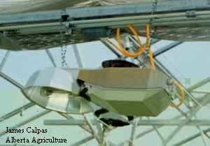
Figure 16. High pressure sodium light.
Temperature Management
Development and flowering of plants relates to both root zone and air temperature (Khah and Passam 1992), and control of temperature is an important tool for the control of crop growth (De Koning 1996).
Managing air temperatures
The optimum temperature is determined by the processes involved in the utilization of assimilate products of photosynthesis, ie. distribution of dry matter to shoots, leaves, roots and fruit (De Koning 1996). For the control of crop growth, average temperature over one or several days is more important than the day/night temperature differences (Bakker 1989, De Koning 1996). This average temperature is also referred to as the 24-hour average temperature or 24-hour mean temperature (Bakker 1989, Portree 1996). Various greenhouse crops show a very close relationship between growth, yield and the 24-hour mean temperature (Bakker 1989, Portree 1996).
With the goal of directing growth and maintaining optimum plant balance for sustained high yield production, the 24-hour mean temperature can be manipulated to direct the plant to be more generative in growth, or more vegetative in growth. Optimum photosynthesis occurs between 21 to 22 �C (Portree 1996), this temperature serves as the target for managing temperatures during the day when photosynthesis occurs. Optimum temperatures for vegetative growth for greenhouse peppers is between 21 to 23 �C, with the optimum temperature for yield about 21 �C (Bakker 1989). Fruit set, however, is determined by the 24-hour mean temperature and the difference in day - night temperatures (Bakker 1989), with the optimum night temperature for flowering and fruit setting at 16 to 18 �C (Pressman 1998). Target 24-hour mean temperatures for the main greenhouse vegetable crops (cucumbers, tomatoes, peppers) can vary from crop to crop with differences even between cultivars of the same crop.
The 24-hour mean temperature optimums for vegetable crops range between 21 to 23 �C, depending on light intensity. The general management strategy for directing the growth of the crop is to raise the 24-hour average temperature to push the plants in a generative direction and to lower the 24-hour average temperature to encourage vegetative growth (Portree 1996). Adjustments to the 24-hour mean temperature are made usually within 1 to 1.5 degrees Celsius with careful attention paid to the crop response.
One assumption that is made when using air temperature as the guide to directing plant growth is that it represents the actual plant temperature. The role of temperature in the optimization of plant performance and yield is ultimately based on the temperature of the plants. Plant temperatures are usually within a degree of air temperature, however during the high light periods of the year, plant tissues exposed to high light can reach 10 to 12 �C higher than air temperatures. It is important to be aware of this fact and to use strategies such as shading and evaporative cooling to reduce overheating of the plant tissues. Infrared thermometers are useful for determining actual leaf temperature.
Precision heat in the canopy
Precision heating of specific areas within the crop canopy add another dimension of air temperature control beyond maintaining optimum temperatures of the entire greenhouse air mass. Using heating pipes that can be raised and lowered, heat can be applied close to flowers and developing fruit to provide optimum temperatures for maximum development in spite of the day - night temperature fluctuations required to signal the plant to produce more flowers. The rate of fruit development can be enhanced with little effect on overall plant development and flower set (De Koning 1996). Precise application of heat in this manner can avoid the problem of low temperatures to the flowers and fruit which are known to disturb flowering and fruit set (Bakker 1989). The functioning of pepper flowers are affected below 14 �C , the number of pollen grains per flower are reduced and fruit set under low night temperatures are generally deformed (Pressman 1998). Problems with low night temperatures can be sporadic in the greenhouse during the cold winter months and can occur even if the environmental control system is apparently meeting and maintaining the set optimum temperature targets. There can be a number of reasons for this, but the primary reasons are 1) lags in response time between the system's detection of the heating setpoint temperature and when the operation of the system is able to provide the required heat throughout the greenhouse and 2) specific temperature variations in the greenhouse due to drafts and "cold pockets".
Managing root zone temperatures
Root zone temperatures are primarily managed to remain in a narrow range to ensure proper root functioning. Target temperatures for the root zone are 18 to 21 �C. Control of the root zone temperature is primarily a concern for Alberta growers in winter, and is obtained through the use of bottom heat systems such as pipe and rail systems. Control is maintained by monitoring the temperature at the roots and maintaining the pipe at a temperature that ensures optimum root zone temperatures.
The use of tempered irrigation water is also a strategy employed by some growers. Maintaining warm irrigation water (20 �C is optimum) minimizes the shock to the root system associated with the delivery of cold irrigation water. In cases during the winter months, in the absence of a pipe and rail system, root zone temperatures can drop to 15 �C or lower. The performance of most greenhouse vegetable crops is sub optimal at this low root zone temperature. Using tempered irrigation water alone is not usually successful in raising and maintaining root zone temperatures to optimum levels. The reasons for this are two fold; firstly, the volume of water required for irrigation over the course of the day during the winter months is too small to allow for the adequate sustained warming of the root zone, and secondly, the temperature of the irrigation water would have to be almost hot in order to effect any immediate change in root zone temperature. Root injury can begin to occur at temperatures in excess of 23 �C in direct contact with the roots. The recommendation for irrigation water temperature is not to exceed 24 - 25 �C. The purpose of the irrigation system is to optimize the delivery of water and nutrients to the root systems of the plants, using it for any other purpose generally compromises the main function of the irrigation system.
Systems for controlling root zone temperatures are primarily confined to providing heat during the winter months. During the hot summer months temperatures in the root zone can climb to over 25 �C if the plants are grown in sawdust bags or rockwool slabs, and if the bags are exposed to prolonged direct sunlight. Avoiding high root zone temperatures is accomplished primarily by ensuring an adequate crop canopy to shade the root system. Also, since larger volumes of water are applied to the plants during the summer, ensuring that the irrigation water is relatively cool, approximately 18 �C, (if possible) will help in preventing excessive root zone temperatures. One important point to keep in mind with respect to irrigation water temperatures during the summer months is irrigation pipe exposed to the direct sun can cause the standing water in the pipe to reach very high temperatures, in excess of 35 �C! Irrigation pipe is often black to prevent light penetration into the line which can result in the development of algae and the associated problems with clogged drippers. It is important to monitor irrigation water temperatures at the plant dripline, especially during the first part of the irrigation cycle, to ensure that the temperatures are not too high. All exposed irrigation pipe should be shaded with white plastic or moved out of the direct sunlight if a problem is detected.
Management of the Relative Humidity Using Vapour Pressure Deficits
Plants exchange energy with the environment primarily through the evaporation of water, through the process of transpiration (Papadakis et al 1994). Transpiration is the only type of transfer process in the greenhouse that has both a physical and biological basis (Papadakis et al 1994). This plant process is almost exclusively responsible for the subtropical climate in the greenhouse (Papadakis et al 1994). Seventy percent of the light energy falling on a greenhouse crop goes towards transpiration, the changing of liquid water to water vapour (Hanan 1990), and most of the irrigation water applied to the crop is lost through transpiration (Papadakis et al 1994).
Relative humidity (RH) is a measure of the water vapour content of the air. The use of relative humidity to measure the amount of water in the air is based on the fact that the ability of the air to hold water vapour is dependent on the temperature of the air. Relative humidity is defined as the amount of water vapour in the air compared to the maximum amount of water vapour the air is able to hold at that temperature (Tilley 1979, Portree 1996). The implication of this is that a given reading of relative humidity reflects different amounts of water vapour in the air at different temperatures. For example air at a temperature of 24 �C at a RH of 80% is actually holding more water vapour than air at a temperature of 20 �C at a RH of 80%.
The use of relative humidity for control of the water content of the greenhouse air mass has commonly been approached by maintaining the relative humidity below threshold values, one for the day and one for the night (Stanghellini and Van Meurs 1992). This type of humidity control was directed at preserving low humidity (Stanghellini and Van Meurs 1992), and although humidity levels high enough to favour disease organisms must be avoided (Stanghellini and Van Meurs 1992), there are more optimal approaches to control the humidity levels in the greenhouse environment. The sole use of relative humidity as the basis of controlling greenhouse air water content does not allow for optimization of the growing environment, as it does not provide a firm basis for dealing with plant processes such as transpiration in a direct manner. (Hanan 1990). The common purpose of humidity control is to sustain a minimal rate of transpiration (Stanghellini and Van Meurs 1992).
The transpiration rate of a given greenhouse crop is a function of three in-house variables: temperature, humidity and light (Stanghellini and Van Meurs 1992, Van Meurs and Stanghellini 1992). Light is the one variable usually outside the control of most greenhouse growers. If the existing natural light levels are accepted, then crop transpiration is primarily determined by the temperature and humidity in the greenhouse (Stanghellini and Van Meurs 1992). Achievement of the optimum "transpiration setpoint" depends on the management of temperature and humidity within the greenhouse. More specifically, at each level of natural light received into the greenhouse, a transpiration setpoint should allow for the determination of optimal temperature and humidity setpoints (Stanghellini and Van Meurs 1992).
The relationship between transpiration and humidity is awkward to describe, as it is largely related to the reaction of the stomata to the difference in vapour pressure between the leaves and the air (Stanghellini and Van Meurs 1992). The most certain piece of knowledge about how stomata behave under increasing vapour pressure difference is it is dependent on the plant species in question (Stanghellini and Van Meurs 1992). However, even with the current uncertainties with understanding the relationships and determining mechanisms involved, the main point to remember about environmental control of transpiration is that it is possible (Stanghellini and Van Meurs 1992, Van Meurs and Stanghellini 1992).
The concept of vapour pressure difference or vapour pressure deficit (VPD) can be used to establish setpoints for temperature and relative humidity in combination to optimize transpiration under any given light level. VPD is one of the important environmental factors influencing the growth and development of greenhouse crops (Zabri and Burrage 1997), and offers a more accurate characteristic for describing water saturation of the air than relative humidity because VPD is not temperature dependent (Rodov et al 1995). Vapour pressure can be thought of as the concentration, or level of saturation of water existing as a gas, in the air (Tilley 1979). As warm air can hold more water vapour than cool air, so the vapour pressures of water in warm air can reach higher values than in cool air. There is a natural movement from areas of high concentration to areas of low concentration. Just as heat naturally flows from warm areas to cool areas, so does water vapour move from areas of high vapour pressure, or high concentration, to areas of low vapour pressure, or low concentration. This is true for any given air temperature. The vapour pressure deficit is used to describe the difference in water vapour concentration between two areas. The size of the difference also indicates the natural "draw" or force driving the water vapour to move from the area of high concentration to low concentration. The rate of transpiration, or water vapour loss from a leaf into the air around the leaf, can be thought of, and managed using the concept of vapour pressure deficit (VPD). Plants maintained under low VPD had lower transpiration rates while plants under high VPD can experience higher transpiration rates and greater water stress (Zabri and Burrage 1997).
A key point when considering the concept of VPD as it applies to controlling plant transpiration is the vapour pressure of water vapour is always higher inside the leaf than outside the leaf. Meaning the concentration of water vapour is always greater within the leaf than in the greenhouse environment, with the possible exception of having a very undesirable 100% relative humidity in the greenhouse environment. This means the natural tendency of movement of water vapour is from within the leaf into the greenhouse environment. The rate of movement of water from within the leaf into the greenhouse air, or transpiration, is governed largely by the difference in the vapour pressure of water in the greenhouse air and the vapour pressure within the leaf. The relative humidity of the air within the leaf can be considered to always be 100% (Papadakis et al 1994), so by optimizing temperature and relative humidity of the greenhouse air, growers can establish and maintain a certain rate of water loss from the leaf, a certain transpiration rate. The ultimate goal is to establish and maintain the optimum transpiration rate for maximum yield. Crop yield is linked to the relative increase or decrease in transpiration, a simplified relationship relates increase in yield to increase in VPD (Jolliet et al 1993)
Transpiration is a key plant process for cooling the plant, bringing nutrients in from the root system and for the allocation of resources within the plant. Transpiration rate can determine the maximum efficiency by which photosynthesis occurs, how efficiently nutrients are brought into the plant and combined with the products of photosynthesis, and how these resources for growth are distributed throughout the plant. Since the principles of VPD can be used to control the transpiration rate, there is a range of optimum VPDs corresponding to optimum transpiration rates for maximum sustained yield (Portree 1996).
The measurement of VPD is done in terms of pressure, using units such as millibars (mb) or kilopascals (kPa) or units of concentration, grams per cubic meter (g/m3). The units of measurement can vary from sensor to sensor, or between the various systems used to control VPD. The optimum range of VPD is between 3 to 7 grams/m3 (Portree 1996), and regardless of how VPD is measured, maintaining VPD in the optimum range can be obtained by meeting specific corresponding relative humidity and temperature targets. Table 1 presents the temperature - relative humidity combinations required to maintain the range of optimal VPD in the greenhouse environment. It is important to remember that this table only displays the temperature and humidity targets to obtain the range of optimum VPDs, it does not consider the temperature targets that are optimal for specific crops. There is a range of optimal growing temperatures for each crop that will determine a narrower band of temperature - humidity targets for optimizing VPD.
Table 1. Relative Humidity and Temperature Targets to Obtain Optimal Vapour Pressure Deficits Gram/m3* and millibars (mb) Relative Humidity
Temp
oC | 95% | 90 % | 85 % | 80 % | 75 % | 70 % | 65 % | 60 % | 55 % | 50 % |
| gm/m3 | mb | gm/m3 | mb | gm/m3 | mb | gm/m3 | mb | gm/m3 | mb | gm/m3 | mb | gm/m3 | mb | gm/m3 | mb | gm/m3 | mb | gm/m3 | mb |
| 15 | 0.5 | 0.6 | 1.1 | 1.4 | 1.7 | 2.2 | 2.2 | 2.9 | 2.8 | 3.7 | 3.3 | 4.3 | 3.9 | 5.1 | 4.4 | 5.8 | 5.0 | 6.6 | 5.5 | 7.2 |
| 16 | 0.6 | 0.8 | 1.2 | 1.6 | 1.8 | 2.4 | 2.3 | 3.0 | 2.9 | 3.8 | 3.5 | 4.6 | 4.1 | 5.4 | 4.7 | 6.2 | 5.3 | 7.0 | 5.8 | 7.6 |
| 17 | 0.6 | 0.8 | 1.3 | 1.7 | 1.9 | 2.5 | 2.5 | 3.3 | 3.1 | 4.1 | 3.7 | 4.9 | 4.3 | 5.6 | 5.0 | 6.6 | 5.6 | 7.4 | 6.2 | 8.1 |
| 18 | .07 | 0.9 | 1.3 | 1.7 | 2.0 | 2.6 | 2.7 | 3.6 | 3.3 | 4.3 | 4.0 | 5.3 | 4.6 | 6.1 | 5.3 | 7.0 | 5.9 | 7.8 | 6.6 | 8.7 |
| 19 | .07 | 0.9 | 1.4 | 1.8 | 2.1 | 2.8 | 2.9 | 3.8 | 3.6 | 4.7 | 4.3 | 5.6 | 5.0 | 6.6 | 5.7 | 7.5 | 6.4 | 8.4 | 7.1 | 9.3 |
| 20 | .08 | 1.0 | 1.5 | 2.0 | 2.2 | 2.9 | 3.0 | 3.9 | 3.8 | 5.0 | 4.5 | 5.9 | 5.3 | 7.0 | 6.1 | 8.0 | 6.8 | 8.9 | 7.5 | 9.9 |
| 21 | .08 | 1.0 | 1.6 | 2.1 | 2.4 | 3.2 | 3.3 | 4.3 | 4.1 | 5.4 | 4.9 | 6.4 | 5.7 | 7.5 | 6.5 | 8.6 | 7.3 | 9.6 | 8.1 | 10.7 |
| 22 | .09 | 1.2 | 1.7 | 2.2 | 2.6 | 3.4 | 3.5 | 4.6 | 4.3 | 5.7 | 5.2 | 6.8 | 6.0 | 7.9 | 6.8 | 8.9 | 7.7 | 10.1 | 8.6 | 14.8 |
| 23 | .09 | 1.2 | 1.8 | 2.4 | 2.7 | 3.6 | 3.7 | 4.9 | 4.6 | 6.1 | 5.5 | 7.2 | 6.4 | 8.4 | 7.4 | 9.7 | 8.3 | 10.9 | 9.2 | 12.1 |
| 24 | 1.0 | 1.3 | 2.0 | 2.6 | 3.0 | 3.9 | 3.9 | 5.1 | 4.9 | 6.4 | 5.8 | 7.6 | 6.8 | 8.9 | 7.8 | 10.3 | 8.8 | 11.6 | 9.7 | 12.7 |
| 25 | 1.0 | 1.3 | 2.0 | 2.6 | 3.0 | 3.9 | 4.1 | 5.4 | 5.2 | 6.8 | 6.2 | 8.1 | 7.2 | 9.5 | 8.2 | 10.7 | 9.2 | 12.1 | 10.3 | 13.6 |
| 26 | 1.1 | 1.4 | 2.2 | 2.9 | 3.3 | 4.3 | 4.4 | 5.8 | 5.5 | 7.2 | 6.6 | 8.7 | 7.7 | 10.1 | 8.8 | 11.6 | 9.9 | 13.0 | 11.0 | 14.5 |
| 27 | 1.2 | 1.6 | 2.4 | 3.2 | 3.6 | 4.7 | 4.7 | 6.2 | 5.9 | 7.8 | 7.1 | 9.3 | 8.3 | 10.9 | 9.4 | 12.3 | 10.6 | 13.9 | 11.7 | 15.4 |
| 28 | 1.3 | 1.7 | 2.5 | 3.3 | 3.7 | 4.9 | 5.0 | 6.6 | 6.3 | 8.3 | 7.5 | 9.9 | 8.7 | 11.4 | 9.9 | 13.0 | 11.2 | 14.7 | 12.4 | 16.3 |
| 29 | 1.4 | 1.8 | 2.7 | 3.6 | 4.1 | 5.4 | 5.3 | 7.0 | 6.7 | 8.8 | 8.0 | 10.1 | 9.3 | 12.2 | 10.8 | 14.2 | 11.9 | 15.6 | 13.2 | 17.4 |
| 30 | 1.4 | 1.8 | 2.8 | 3.7 | 4.2 | 5.5 | 5.7 | 7.5 | 7.1 | 9.3 | 8.5 | 11.2 | 9.9 | 13.0 | 11.3 | 14.8 | 12.7 | 16.7 | 14.0 | 18.4 |
*Optimum range 3-7 grams/m3, 3.9-9.2 mb
The plants themselves exert tremendous influence on the greenhouse climate (Lange and Tantau 1996), transpiration not only serves to add moisture to the environment, but is also the mechanism by which plants cool themselves and add heat to the environment (Papadakis et al 1994). Optimization of transpiration rates through management of air temperature and relative humidity can change over the course of the season. Early in the season, when plants are young and the outside temperatures are cold, both heat and humidity (from mist systems) can be applied to maintain temperature and humidity targets. As the season progresses and the crop matures, increasing light intensity increases the transpiration rate and the moisture content of the air. To maintain optimum rates of transpiration, venting is employed to reduce the relative humidity in the air. However, under typical summer conditions in Alberta, particularly in the south, ventilation is almost exclusively triggered by high temperature setpoints calling for cooling. Under these conditions, ventilation can occur continuously throughout the daylight period and results in very low relative humidity in the greenhouse. As the hot, moist air is vented, it is replaced by still warm, dry air. Southern Alberta is a dry environment with the relative humidity of the air in summer routinely falling below 30%. Under these conditions some form of additional cooling, mist systems or pad and fan evaporative cooling, is required to both reduce the amount of ventilation for cooling as well as to add moisture to the air.
Carbon Dioxide Supplementation
Carbon dioxide (CO2) is one of the inputs of photosynthesis and as such CO2 plays an important role in increasing crop productivity (Hand 1993, Rijkdjik and Houter 1993). Optimal CO2 concentrations for the greenhouse atmosphere fall with the range of between 700 to 900 ppm (parts per million) (Romero-Aranda et al 1995, Tremblay and Gosselin 1998). Crop productivity depends not only on efficiency of interception of light but also on the efficiency with which light is converted to chemical energy in photosynthesis. Carbon dioxide enrichment to 1200 ppm increases the maximum conversion efficiency by a substantial amount (between 28 to 59%) (Wilson et al 1992). Photosynthetic efficiencies appear never to exceed about 22 % of the absorbed light energy in the 400 to 700 nm range, the maximum efficiency is obtained at relative low light intensities, not in brightest sunlight (Salisbury and Ross 1978). Considering the supply of light to available land area on which a crop is growing, the overall yield efficiencies are always much below 22% (Salisbury and Ross 1978). The use of CO2 in greenhouses can give light use efficiencies exceeding those of field crops (Wilson et al 1992). Glasshouse crops with CO2 enrichment achieve maximum efficiency of light energy utilization between 12-13% (Wilson et al 1992). The ability of plants to utilize CO2 is dependent upon the presence of light, for this reason it is only useful to supplement CO2 during the daylight hours (Styer and Koranski 1997).
The key enzyme for CO2 fixation is rubisco (Tremblay and Gosselin 1998). The activity of rubisco depends on the ratio of the O2 and CO2 concentration in the atmosphere (Tremblay and Gosselin 1998). The major effect of CO2 enrichment is the shift in balance in the O2 and CO2 ratio which improves the activity of rubisco (Tremblay and Gosselin 1998). The effect is just as important at low as at high light levels since the percentage effect on relative growth rate is about the same over a range of light levels (Tremblay and Gosselin 1998). Transpiration rates are reduced under CO2 enrichment conditions by 34%. Increased net leaf photosynthesis rate and decreased transpiration rate under CO2 enrichment is well documented. One of the most important effects of CO2 enrichment is the increased water use efficiency (Tremblay and Gosselin 1998).
The technique of enriching the greenhouse atmosphere with CO2 to maximize yield is standard practice (Slack et al 1988, Nederhof et al 1992, Rijkdijk and Houter 1993). The largest increase in growth rate achieved with CO2 enrichment is obtained with high light intensities. A high CO2 concentration may partially compensate for low light levels (Fierro et al 1994). There is obviously a potential for synergism between CO2 and light, however the relationship between CO2 and light conditions may be relatively loose (Tremblay and Gosselin 1998).
When greenhouse ventilation rates are high, the cost of CO2 supplementation can rise steeply. This is particularly so with a ventilation regime where ventilation is triggered at temperatures between 19 - 21 �C (Slack et al 1988). Investigations into delaying ventilation to increase the cost effectiveness of CO2 supplementation have shown that the amounts of CO2 supplied to the greenhouse could be reduced by 23 to 35% while still maintaining the CO2 content of the greenhouse atmosphere above ambient CO2 concentrations (Slack et al 1988). Delaying ventilation to conserve CO2 resulted in higher greenhouse temperatures with fruit temperatures exceeding 30 �C. However, total marketable yield fell by 11% and the proportion of fruit graded as Class 1 was reduced by 20% on average (Slack et al 1988).
The best advice for CO2 supplementation under high ventilation rates is to maintain the CO2 concentration at or just above the normal ambient level of approximately 350 ppm (Slack et al 1988). This is a highly efficient way of using CO2 supplementation. Maintaining the CO2 concentration at the same level as ambient, there can be no net exchange of CO2 with the outside air through leakage or ventilation (Slack et al 1988). For practical purposes, the input of CO2 is therefore equal to that being assimilated by the crop during photosynthesis, i.e. the utilization of supplementary CO2 is totally efficient (Slack et al 1988). The main point being that ventilation and economical CO2 enrichment may be applied simultaneously. (Shina and Seginer 1989 Tremblay and Gosselin 1998).
At higher temperatures, 25 �C, net photosynthesis begins to decline and the supplementation of CO2 above this temperature is not considered cost effective (Portree 1996). During longer periods of elevated CO2 the stomata remain partially closed and the reduction of transpiration may cause insufficient cooling, hence, heat damage to the leaves under conditions of intense light (Nederhoff et al 1992). However, the increased VPD associated with the higher temperatures has been shown to counteract the effect of stomatal closure due to CO2 supplementation (Nederhoff et al 1992).
Since young plants grow nearly exponentially, they can benefit more from optimal growing conditions than mature plants (Tremblay and Gosselin 1998). Carbon dioxide enrichment results in heavier transplants and can be used to accelerate the growth, as well as improving the quality of the transplants (Tremblay and Gosselin 1998). Carbon dioxide may increase sugar translocation in the roots as well as facilitating the movement of nitrogen and carbon compounds directed towards the development of new roots (Tremblay and Gosselin 1998). In short, CO2 supplementation shortens the nursery period and results in sturdier, higher quality plants (Tremblay and Gosselin 1998).
Air Pollution in the Greenhouse
Air pollutants can be a concern for greenhouse production. The incidence of air pollutant injury to plants is increasing as more growers use double plastic greenhouses, or other forms of greenhouse sealing to reduce energy loss (Blom 1998). Air pollutants can cause visible injury to the leaves, can reduce growth rates or both (Blom 1998). Tomatoes and cucumbers are particularly sensitive to air pollutant injury (Portree 1996). When considering the effects of greenhouse air pollutants ,it is important to remember that these pollutants pose significant health risks for people working the crops.
Common pollutants are often by-products of combustion. Although sources of pollutants can be outside the greenhouse, a number of sources of pollutants can be found within the greenhouse. Pollutants can be produced by direct-fired heating units, gas supply lines or carbon dioxide generators that burn hydrocarbon fuels such as natural gas (Blom 1998). Significant sources of pollutants outside the greenhouse can include industrial plants or vehicle exhaust (Blom 1998).
Table 2. Maximum acceptable concentration (ppm) of some noxious gases for humans and plants
| Gas | Humans | Plants |
| Carbon Dixoide (CO2) | 5,000 | 4,500 |
| Carbon monoxide (CO) | 47 | 100 |
| Sulfur dioxide (SO2) | 3.5 | 0.1 |
| Hydrogen sulfide (H2S) | 10.5 | 0.01 |
| Ethylene (C2H4) | 5.0 | 0.01 |
| Nitrous oxide (NO) | 5.0 | 0.01 to 0.1 |
| Nitrogen dioxide (NO2) | 5.0 | 0.2 to 2.0 |
| Adapted from Portree 1996 |
Air pollution from sources within the greenhouse commonly arise through cracked heat exchangers on furnaces or incomplete combustion in the furnace or CO2 generators. Heaters and generators should be checked at the beginning of the cropping season to ensure they are operating properly and complete combustion is occurring. The most common air pollutants resulting from incomplete combustion include nitrogen oxides, nitric oxide (NO) and nitrogen dioxide (NO2), sulfur dioxide (SO2), ethylene (C2H4), propylene (C3H6), ozone (O3), carbon monoxide (CO) and hydrogen sulfide (H2S) (Portree 1996, Blom 1998).
Symptoms of air pollutant injury vary with the specific gases involved. The common symptoms of sulfur dioxide injury is characterized by severe leaf burn appearing within 24 to 36 hours of exposure to high levels of the gas (Blom 1998). There is a distinct line between the affected and unaffected areas on the leaves and young leaves are more susceptible to injury than mature leaves (Blom 1998). Symptoms of NO2 injury include darker than normal green leaves with downward curling leaf margins and dead areas on the leaves in severe cases (Blom 1998). Ethylene functions as a plant growth regulator, involved in seed germination, root development, flower development and leaf abscission (Salisbury and Ross 1978, Blom 1998). Ethylene injury can include a reduction in growth, shortening and thickening of stems and twisting of stems, as well as premature leaf and flower drop (Blom 1998). Propylene injury is similar to ethylene but usually occurs at concentrations 100 times higher than those for ethylene (Blom 1998). Ozone injury is characterized by mottling, necrotic flecking or bronzing necrosis of leaves, premature leaf drop and decreased growth (Blom 1998).
Growing Media
Most commercial vegetable production greenhouses in Alberta use some form of "hydroponic culture". The term hydroponics essentially translates as 'water culture'. It is an advanced form of crop culture which allows for specific control of the delivery of nutrients to the plants (Salisbury and Ross 1978, Weiler and Sailus 1996). The term hydroponics can bring to mind a number of variations on the same theme. Hydroponic growing systems can include: substrate culture where the roots are allowed to grow in an inert or semi-inert media; solution culture where the roots are immersed in ponds of nutrient solution; NFT culture (nutrient film technique) where the roots are contained such that a thin film of nutrient solution constantly runs by the roots; and aeroponics where the root systems are suspended within an enclosed area and are misted with nutrient solution (Weiler and Sailus 1996). A general working definition of hydroponic culture that would include all of the above systems, is plant culture where the plants receive fertilizer nutrients every time they receive water.
Using this working definition of hydroponics also leaves room for the inclusion of soil as a growing medium. However, soil culture is not widely practiced in commercial vegetable greenhouses in Alberta. The main reason for moving out of soil, into soilless culture, is to escape problems due to soil borne diseases (Maree 1994, Portree 1996) that can build-up in the soil used year after year. Soilless media such as rockwool and sawdust offer an initially disease-free growing medium. There are other advantages of moving the root system out of the soil and into confined spaces such as sawdust bags or rockwool slabs. The main advantages are realized in the improved management of watering and nutrition, topics which are discussed in more detail in following sections.
Media for seeding and propagation
Rockwool plugs are the most common media used for seeding. Rockwool is manufactured by subjecting rock mineral materials to very high temperatures and then spinning the materials into a fibre (Portree 1996). The plugs can be square (2 cm x 2 cm by 4 cm deep) and can come joined together as a rockwool "flat" that fit into standard 28 cm x 54 cm plastic seeding flats. As the seed germinates and the seedlings are ready for their first transplanting, the plugs easily separate from each other when the seedlings are transplanted into rockwool blocks.
Rock wool blocks are typically around 10 cm x 10 cm by 8 cm deep, with a depression cut into the upper surface to receive the rockwool plug at the first transplanting. As the seedling continues to grow, the root system develops from the rockwool plug into the confines of the block. When the seedling is ready for transplanting into the main production greenhouse at "house set", the bottom of the rockwool block is placed in direct contact with the larger volume of growing media used in the production house.
Growing media for the production greenhouse
The majority of Alberta's commercial greenhouse vegetable production is based on substrate culture where the plants are grown in sawdust or rockwool. These substrates contain practically nothing in the way of plant nutrients and serve as a substrate for the root system to anchor the plant. The growing media plays a significant role in defining the environment of the root system and allows for the transfer of water and nutrients to the plant. Typically, for sawdust culture, 2 or 3 plants are grown in 20 to 25 litre white plastic bags (white reflects more light) filled with spruce and/or pine sawdust. Rockwool culture uses approximately 16 litres of rockwool substrate for every 2 to 3 plants (Portree 1996). The sawdust bags or rockwool slabs are placed directly on the white plastic floor of the greenhouse.
Sawdust is less expensive than rockwool in initial cost, however standard density rockwool slabs can be pasteurized and reused for up to three years (Maree 1994, Portree 1996). Sawdust is a waste product of the lumber milling process which is usually burned, so the use of sawdust as a growing media is an environmentally sound practice. For sawdust culture it is important to use a moderately fine sawdust, lumber mills in Alberta understand the sawdust requirements for plant production and will supply "horticultural grade" sawdust if they are made aware that the sawdust is to be used for plant culture. Using sawdust that is too fine will break down over the production season with resulting loss of airspace around the roots which can lead to root death (Benoit and Ceustermans 1994, Portree 1996).
There is always some decomposition of the sawdust during the growing season (Benoit and Ceustermans 1994) which makes the product useful for further composting or adding to mineral soils to improve soil quality. Through the continued action of soil microbes the sawdust residue at the end of the cropping season is returned to the environment in an ecologically sound manner. The waste from sawdust culture is confined to the plastic bags themselves which are recovered when the sawdust bags are dumped and can be recycled where facilities exist.
Management of Irrigation and Fertilizer Feed
In hydroponic crop production systems the application of water is integrated with the application of the fertilizer feed. The management of fertilizer application to the plants is therefore integrated with the management of watering. The management of watering and nutrition is focused on the optimal delivery of water and nutrients over the various growth stages of the plant, through the changing growing environment over the production year, in order to maximize yield.
Water quality
Plants are comprised of 80 to 90% water (Salisbury and Ross 1978) and the availability of adequate quality water is very important to successful crop production (Portree 1996, Styer and Koranski 1997). The quality of water is determined by what is contained in the water at the source; well, dugout, town or city water supply, and the acidity or alkalinity of the water. Water is a solvent, and as such, it can contain or hold a certain quantity of soluble salts in solution. Fertilizers, by their nature, are soluble salts, and growers dissolve fertilizers in water to obtain nutrient solutions in order to provide the plants with adequate nutrition. Prior to using any source of water for crop production it is important to have it tested for quality. Water quality tests determine the amount of various salts commonly associated with water quality concerns. The maximum desirable concentrations, in parts per million (ppm), for specific salt ions in water for greenhouse crop production are presented in table 3. Parts per million are one unit of measurement of the amount of dissolved ions, or salt in water, and are also used to measure the level of dissolved fertilizer salts in nutrient solutions. The level of nutrients as dissolved ions in water can also be reported in milligrams/Litre of solution. There is a direct relationship between milligrams/Litre (mg/L) and ppm, where 1 mg/L = 1 ppm. Another common unit of measure for dissolved fertilizer salts is the millimole (mM), the concept of millimoles and the relationship between millimoles and ppm is explained in the special topic section.
1 mmho/cm = 1 mS/cm = 1000 microsiemens/cm
Figure 17. The relationship between common units of measurement for electrical conductivity (E.C.)
Table 3. The maximum desirable concentrations, in parts per million (ppm), for specific salt ions in water for greenhouse crop production.
| Element | Maximum desirable (ppm) |
| Nitrogen (NO3 - N) | 5 |
| Phosphorus (H2PO4 - P) | 5 |
| Potassium (K+) | 5 |
| Calcium (Ca++) | 120 |
| Magnesium (Mg++) | 25 |
| Chloride (Cl-) | 100 |
| Sulphate (SO4--) | 200 |
| Bicarbonate (HCO3-) | 60 |
| Sodium (Na++) | 30 |
| Iron (Fe+++) | 5 |
| Boron (B) | 0.5 |
| Zinc (Zn++) | 0.5 |
| Manganese (Mn++) | 1.0 |
| Copper (Cu++) | 0.2 |
| Molybdenum (Mo) | 0.02 |
| Fluoride (F-) | 1 |
 | |
| pH | 75 |
| |
| E.C. | 1 |
Water quality tests will also report the pH, the acidity or alkalinity of the water. Once the source of water has been determined as suitable for greenhouse crop production it is also important to have the water tested routinely to ensure that any fluctuations in quality that may occur does not compromise crop production.
Electrical conductivity of water
Water quality analyses also report the electrical conductivity or E.C. of the water. The ability of water to conduct an electrical current is dependent of the amount of ions or salts dissolved in the water. The greater the amount of dissolved salts in the water, the more readily the water will conduct electricity. Electrical conductivity is an indirect measurement of the level of salts in the water and can be a useful tool for both determining the general suitability of water for crop production, and for the ongoing monitoring of the fertilizer feed solution. Using electrical conductivity as a measure to maintain E.C. targets in the nutrient solution and the root zone can be used as a management tool for making decisions regarding the delivery of fertilizer solution to the plants.
Electrical conductivity is measured and reported using a number of measurement units including millimhos per centimeter (mmhos/cm), millisiemens per centimeter (mS/cm) or microsiemens per centimeter. Water suitable for greenhouse crop production should not have a E.C. in excess of 1.0 mmhos/cm.
pH
The relative acidity and alkalinity of the water is expressed as pH (Styer and Koranski 1997), and is measured on a scale from 0 to 14. The lower the number, the more acidic the water or solution, the higher the number the more alkaline (Boikess and Edelson 1981). The pH scale is a logarithmic scale, meaning that every increase of one number ie. 4 to 5, represents a ten times increase in alkalinity. Conversely, every single number decrease, ie. 5 to 4, represents a ten times increase in acidity.
Most water supplies in Alberta are alkaline, with typical pH levels of 7.0 to 7.5. Alkalinity of the water increases with increasing levels of bicarbonate. The pH measurement reflects the chemistry of the water and nutrient solution. The pH of a fertilizer solution has a dramatic determining effect on the solubility of nutrients, how available the nutrients are to the plant (Portree 1996, Styer and Kornaski 1997).
The optimum pH of a feed solution, with respect to the availability of nutrients to plants, falls within the range of 5.5 to 6.0 (Portree 1996). The pH of a solution can be adjusted through the use of acids such as phosphoric or nitric acid, or potassium bicarbonate, depending on which direction the feed solution needs to be adjusted. When acids or bases are used to adjust the pH of the feed solution, the nutrients added by the acid; nitrogen, phosphorus, must be accounted for when the feed solution is calculated. Most water supplies in Alberta are basic in pH and require the use of acid for pH correction.
The amount of acid required to adjust the pH is usually dependent on the bicarbonate (HCO3-) level in the water. The amount of bicarbonate in the water supply can be determined by a water analysis, and is reported in ppms. A good target pH for nutrient feed solution is 5.8, and as a general rule this pH corresponds to a bicarbonate level of about 60 ppm. If the incoming water has, for example, a pH of 8.1 and a bicarbonate level reported at 207 ppm, 207 ppm - 60 ppm = 147 ppm that needs to be neutralized by acid to reduce the pH from 8.1 to 5.8.
In order to neutralize 61 ppm, or 1 milliequivalent, of bicarbonate it takes about 70 ml of 85% phosphoric acid, or about 84 ml of 67% nitric acid per 1000 litres of water. In order to neutralize 147 ppm of bicarbonate:
Using 85% phosphoric acid
140 / 61 = 2.3 milliequivalents of bicarbonate to be neutralized
2.3 milliequivalents x 70 ml of 85% phosphoric acid for each milliequivalent
= 2.3 x 70 ml = 161 mls of 85% phosphoric acid for every 1000 litres of water.
Using 67% nitric acid
2.3 milliequivalents of bicarbonate to be neutralized.
2.3 milliequivalents x 76 ml per milliequivalent
= 2.3 x 76 ml = 175 mls of 67% nitric acid for every 1000 litres of water
These calculations have to be made for each water sample based on the results of water a analysis reporting the level of bicarbonates. In addition to phosphoric and nitric acid, sulfuric and hydrochloric acids can also be used to adjust the pH of the water down.
Acids are corrosive. Special care and attention must be used when handling them for pH correction. The common acids used to lower the pH are phosphoric acid (85%) and nitric acid (67%), of these two, nitric acid is the most corrosive (Styer and Koranski 1997) and must be handled very carefully. Acid resistant safety glasses, rubber gloves and a rubber apron should be the minimum safety equipment used when handling acids.
The mineral nutrition of plants
In order to support optimum growth, development and yield of the crop, the fertilizer feed solution has to continually meet the nutritional requirements of the plants. Although the mineral nutrition of plants is complex, experience in crop culture has determined basic requirements for the successful hydroponic culture of plants. There are 13 mineral elements that are considered essential for plant growth. Water (H2O) and carbon dioxide (CO2) are also necessary for plant growth and supply hydrogen, carbon and oxygen to the plants bringing the total to 16 essential elements (Salisbury and Ross 1978).
Table 4. The essential mineral elements for plants
Element | Symbol | Type | Mobility in Plant | Symptoms of Deficiency |
| Nitrogen | N | macronutrient | mobile | Plant light green, lower (older) leaves yellow. |
| Phosphorus | P | macronutrient | mobile | Plant dark green turning to purple. |
| Potassium | K | macronutrient | mobile | Yellowish green margins on older leaves. |
| Magnesium | Mg | macronutrient | mobile | Chlorosis between the veins on older leaves first, turning to necrotic spots, flecked appearance at first. |
| Calcium | Ca | macronutrient | immobile | Young leaves of terminal bud dying back at tips and margins. Blossom end rot of fruit (tomato and pepper). |
| Sulfur | S | macronutrient | immobile | Leaves light green in color. |
| Iron | Fe | micronutrient | immobile | Yellowing between veins on young leaves (interveinal chlorosis), netted pattern. |
| Manganese | Mn | micronutrient | immobile | interveinal chlorosis, netted pattern |
| Boron | B | micronutrient | immobile | Leaves of terminal bud becoming light green at bases, eventually dying. Plants "brittle." |
| Copper | Cu | micronutrient | immobile | Young leaves dropping, wilted appearance. |
| Zinc | Zn | micronutrient | immobile | interveinal chlorosis of older leaves. |
| Molybdenum | Mo | micronutrient | immobile | Lower leaves pale, developing a scorched appearance. |
A criterion to determine whether an element is essential to plants is if the plant cannot complete its life cycle in the complete absence of the element (Salisbury and Ross 1978). In addition to the essential elements there are other elements, although not necessarily considered universally essential, which can affect the growth of plants. Sodium (Na), chloride (Cl) and silicon (Si) are in this category, all three of these nutrients either enhance the growth of plants, or are considered essential nutrients for some plant species (Wilson and Loomis 1967, Salisbury and Ross 1978, Styer and Koranski 1997).
The essential nutrients can be grouped into two categories reflecting the quantities of the nutrients required by plants. Macronutrients or major elements, are required by plants in larger quantities, when compared to the amounts of micronutrients, or trace elements required for growth (Salisbury and Ross 1978). Another useful grouping of the mineral nutrients is based on the relative ability of the plant to translocate the nutrients from older leaves to younger leaves (Salisbury and Ross 1978). Mobile nutrients are those which can readily be moved by the plant from older leaves to younger leaves, nitrogen is an example of a mobile nutrient (Salisbury and Ross 1978). Calcium is an example of an immobile nutrient, one which the plant is not able to move after it has initially been translocated to a specific location (Salisbury and Ross 1978).
The discussion of plant nutrients as elements does not allow for a more complete discussion of how plants access the elements from the root environment, and how hydroponic growers ensure that their crop plants are adequately supplied with nutrients. The term "element" can be defined as a substance that cannot be broken down into simpler substances by chemical means, the basic unit of an element is the atom (Boikess and Edelson 1981). With the simplest, or purest form of plant nutrients being the atom, nutrients are not often available to plants in their purest form. Pure nitrogen is an example of a nutrient element represented by its atom. When the atoms of different elements combine, they can form other substances which are based on a particular combination of atoms, substances based on molecules. Nitrate (NO3-), is a molecule based on nitrogen and oxygen atoms, nitrate is absorbed by plant roots as a source of nitrogen. Nitrate is an "available" form of nitrogen. The nitrate molecule has an overall negative charge, which causes the molecule to be fairly reactive chemically, and therefore more available.
The availability of nutrient elements to plants is generally based on the existence of the nutrient element as a charged particle, either a charged atom or charged molecule. An atom or molecule that carries an electric charge is called an ion, and positively charged ions are called cations, while negatively charged ions are called anions. The nitrate molecule (NO3-) is an anion, the iron atom can exist as the Fe+2 (ferrous) or Fe+3 (ferric) cations (Boikess and Edelson 1981). Plants are able to acquire the essential mineral elements via the root system utilizing the chemical properties of ions, particularly that to acquire negatively charged anions, the plant roots have sites that are positively charged. The plant is also able to attract positively charged cations to negatively charged sites on the root.
Water is a very important component in the acquisition of nutrient elements by the plants as the nutrient ions only exist when they are in solution, when they are dissolved in water. As solids, the ions generally exist as salts, a salt can be defined as any compound of anions and cations (Boikess and Edelson 1981). In the absence of water, the nutrient ions form compounds with ions of the opposite charge. Anions combine with cations to form a stable solid compound. For example, the nitrate anion (NO3-) commonly combines with the calcium (Ca+2) or potassium (K+) cations forming the larger calcium nitrate Ca(NO3)2 potassium nitrate (KNO3) salt molecules. As salts are added to water, they dissolve, or dissociate into their respective anion and cation components. Once in solution they become available to plants.
An important point to remember is that different salts have different solubilities, that is, some salts readily dissolve in water (highly soluble), and some salts do not. Calcium sulfate (CaSO4) is a relatively insoluble salt and would be a poor choice as a fertilizer because very little of the calcium would go into solution as the calcium cation (Ca++) and be available to plants. Fertilizer salts, by their very nature, are useful because they go into solution readily. In hydroponic culture, greenhouse growers formulate and make a water based nutrient solution by dissolving fertilizer salts.
In addition to existing as salts, some of the micronutrients; iron, zinc, manganese and copper, exist in chelates. A chelate is a soluble product formed when certain atoms combine with certain organic molecules. The sulphate salts of iron, zinc, manganese and copper are relatively insoluble and chelates function to make these mineral nutrients more readily available in quantity to the plants (Boikess and Edelson 1981).
Fertilizer Feed Programs
Fertilizer nutrient solutions are formulated to meet the needs of the plants using a combination of component fertilizer salts. The amounts of the various fertilizers used are dependent on target levels which have been determined to be optimal for the crop in question. Although there is considerable similarity between fertilizer programs for the various vegetable crops, there can be some differences reflecting the different requirements of the crop. In any event, when mixing fertilizer solutions, only high quality water-soluble fertilizers should be used.
Table 5. Forms of mineral nutrient elements that are commonly available to plants
Element | Symbol | Available as | Symbol |
| Macronutrients |
| Nitrogen | N | Nitrate ion
Ammonium ion | NO3-
NH4+ |
| Phosphorus | P | Monovalent phosphate ion
Divalent phosphate ion | H2PO4-
HPO4-2 |
| Potassium | K | Potassium | K+ |
| Calcium | Ca | Calcium ion | Ca+2 |
| Magnesium | Mg | Magnesium ion | Mg+2 |
| Sulfur | S | Divalent sulfate ion | SO4-2 |
| Chlorine | Cl | Chloride ion | Cl- |
|
| Micronutrients |
| Iron | Fe | Ferrous ion
Ferric ion | Fe-2
Fe-3 |
| Manganese | Mn | Manganous ion | Mn+2 |
| Boron | B | Boric acid | H3BO4 |
| Copper | Cu | Cupric ion chelate
Cuprous ion chelate | Cu+2
Cu+ |
| Zinc | Zn | Zinc ion | Zn+2 |
| Molybdenum | Mo | Molybdate ion | MoO4- |
The required nutrient levels, or target nutrient levels of the various essential elements are often expressed as the desired parts per million (ppm) in the final nutrient solution. The recommended nutrient fertilizer feed targets for greenhouse peppers are listed in table 6. Even though all thirteen mineral elements are essential for plant growth and development, nutrient targets for sulfur and chlorine are not listed. The reason for this is adequate amounts of sulfur are obtained from the use of sulfate fertilizers, potassium sulfate or magnesium sulfate. Chloride is assumed to be present in adequate amounts as a contaminant in a number of fertilizers. As the purity of fertilizers has improved, growers will have to pay more attention to ensuring these other elements, particularly chloride, are present in adequate amounts. Once the recommended nutrient targets are known, calculations are made to determine how much of each fertilizer is required in order to meet them.
In order to make these calculations some other basic information is required:
1. The volume of water that will be used to make the feed solution.
2. The types of fertilizers that are available, and the relative amounts of each nutrient present in the fertilizer.
When considering what volume of water to use for the nutrient solution it is first important to understand the delivery of the nutrient solution to the plants as discussed earlier in "Irrigation and fertilizer feed systems."
Every greenhouse must be able to supply water and nutrients on an ongoing basis. During hot, dry Alberta summers, mature pepper plants can use approximately 3.5 to 4.0 litres of water per plant per day, cucumbers can require over 6 litres, tomatoes up to 3 litres. This water always contains fertilizer which is added as the water comes into the greenhouse and before it is pumped to the plants. There are a number of variations on the theme, but some form of fertilizer injection system is used in all commercial scale greenhouses.
Table 6. Nutrient feed targets (ppm) for greenhouse sweet peppers grown in sawdust.
| Nutrient | Target (ppm) |
| Nitrogen | 200 |
| Phosphorus | 55 |
| Potassium | 318 |
| Calcium | 200 |
| Magnesium | 55 |
| Iron | 3.00 |
| Manganese | 0.50 |
| Copper | 0.12 |
| Molybdenum | 0.12 |
| Zinc | 0.20 |
| Boron | 0.90 |
Feed targets and plant balance
The first approach to altering the feed solution in response to a crop that is overly vegetative is to increase the feed E.C. to direct the plants to become more generative and set and fill more fruit. The feed EC can be increased from 2.5 mmhos to approximately 3.0 mmhos over the course of a few days.
Dialing up the feed E.C. increases the absolute amounts of fertilizer nutrients in the feed but does not affect the ratio of the nutrient levels with respect to one another. Increasing the feed E.C. increases the level of fertilizer salts in the root zone, increasing the stress on the plant as it becomes more difficult for the plant to take up water. The plant responds to the stress by putting more emphasis on fruit production, a stressed plant begins preparations for the end, by trying to ensure that the next generation will carry forward. The fruit holds the seed, and in plant terms, developing fruit means that the next generation will survive and carry on. Now plants don't think these things out, but stressing the plant does direct the plant to set more fruit. There is a limit to how far growers can go with this as a successful crop requires having enough vegetative growth to continually fill a high volume of fruit consistently throughout the season.
There is another option available for affecting the vegetative/generative balance of the plants, through manipulation of the nutrient ratios, particularly the nitrogen-potassium ratio.
Typical absolute value, and relative ratio targets for N, K and Ca in vegetable feed programs (E.C. of 2.5 mmhos) for Southern Alberta production conditions
| Crop | Nutrient Targets (ppm) | Nutrient Ratio |
| N | K | Ca | N | K | Ca |
| cucumber | 20
0 | 30
0 | 173 | 1.00 | 1.51 | 0.86 |
| pepper | 21
4 | 31
8 | 200 | 1.00 | 1.48 | 0.93 |
The N:K ratios presented in the table, are all about 1:1.5, increasing the level of potassium, with respect to nitrogen, and increasing the ration to 1:1.7 will direct the plant to be more generative. The reason for this is that nitrogen promotes vegetative growth while potassium promotes mature growth, generative growth. Calcium is also important for promoting strong tissues, fruit, and mature growth. Shifting the feed program to favor potassium over nitrogen will direct the plant to be generative. Calcium is important in the equation in that it should always be approximately equal to the amount of nitrogen. A N:Ca ration of 1:1, works for both tomatoes and peppers, while a N:Ca ratio of 1:0.85 has shown to work well for cucumbers.
Changes to the N:K ratio should be made carefully, the above ratios come from the feed programs of successful Alberta growers and can serve as a guide. The place to start is to determine the ratios in the current feed program and examine the performance of he crop. If it is determined that there is room for improving the balance of the plants, alterations in the nutrient ratios can be undertaken.
Always be aware that many factors influence plant balance: day/night temperature split, 24 hour average temperature, relative humidity and watering. These factors should be optimized before feed ratios are changed. You have to know where the crop is in order to make sound decisions on where it should be, and how to get there.
Due to the large volumes of fertilizer feed solution that can be required daily, it is impractical to make the fertilizer feed on a day to day basis. Instead, the required fertilizers can be mixed in a concentrated form, usually 100 to 200 times the strength that is delivered to the plants. Injectors or ratio feeders are then used to "meter-out" the correct amount of fertilizer into the water which make up the nutrient solution going to the plants. By using concentrated volumes of the fertilizer feed held in "stock tanks" growers are able to reduce the number of fertilizer batches they have to make. Depending on the number of plants in the crop, the size of the stock tanks, and the strength of the concentrate, growers may only have to mix fertilizer once every 2 to 4 weeks.
Designing a fertilizer feed program
The design of a fertilizer feed program is a relatively straight forward process once the nutrient target levels are decided and basic information about the water quality, feed delivery system, and component fertilizers are known. Fertilizer targets and the component fertilizers used to make the fertilizer solution can change over the course of the year depending on the crop and the knowledge of the grower. Often the changes are slight adjustments in the relative proportion of the macronutrients to one another, particularly the nitrogen:phosphorus:potassium (N:P:K) ratio. Changes can also include the addition of alternate forms of a nutrient in question, a common example is the use of ammonium nitrogen (NH4 - N) in addition to nitrate nitrogen (NO3 - N) during the summer months. Ammonium nitrate is the common source of ammonium nitrogen, which is a more readily available form of nitrogen that works to promote vegetative growth. During the summer months a target of approximately 17 ppm of ammonium nitrogen is recommended to help optimize plant balance and crop production.
Moles and millimoles in the greenhouse; Just another couple of rodents? - Just when you thought you had all your rodent problems under control, some greenhouse vegetable growers have been concerned about millimoles and moles. Not to worry, these growers are not referring to four legged moles. Rather they are using another unit of measure to discuss fertilizer feed targets and root zone targets.
So, what exactly is a millimole? A millimole is one thousandth of a mole, and a mole is defined as the amount of a substance of a system which contains as many elementary entities as there are atoms in exactly 12 grams of 12 C (Carbon 12). Now, you were probably expecting that a definition would help clarify the situation, isn't that what definitions are supposed to do? The concept of the mole has come out of stoichiometry, that branch of chemistry which studies the quantities of reactants and products in chemical reactions.
Now a lot of chemists and physicists have argued for a long time over how to measure the masses of individual elements (some of those same elements that growers feed their crops in fertilizer feed solutions) and in 1961 they settled on using the mole. A good way to understand what a mole is and why to use it is to related it to the concept of a dozen. We understand that a dozen is twelve of something, be it cucumbers, eggs or whatever. A mole is 6.02 x 10²³ of some entity, and chemists usually refer to actual molecules of a substance when they talk about moles, although you could have a mole of eggs or a mole of cucumbers. You would be quite the grower to grow a mole of cucumbers, tomatoes or peppers. The number 6.02 x 10²³ , which in long hand is 602 000 000 000 000 000 000 000, is called Avogadro's number after the nineteenth century chemist who did some pioneering work on gases and was largely ignored for his trouble. The lesson here is that if you do something great and are not feeling appreciated for the greatness, someone, far into the future may name a big number after you.
Moles do relate to parts per million (ppm), they are both ways to measure how much of a given nutrient we are dealing with in a fertilizer feed sample, leachate or tissue sample. The difference is that ppm is a measure of mass (e.g. 1 ppm = 1 milligram/litre) and moles measure amounts. One mole of any substance contains Avogadro's number of entities or basic units. Those entities, as mentioned earlier, can be atoms or molecules or whatever you want. When we talk about one mole of nitrate nitrogen, NO3, we are referring to 6.02 x 10²³ molecules of NO3, because the basic NO3 entity is made up of one atom of nitrogen (N) and three atoms of oxygen (O). If we are talking about a mole of iron, Fe, we are talking about atoms, because the basic entity of iron is the iron atom.
All atoms and molecules have different basic weights, some being heavier than other. If we talk about 1 ppm of NO3 versus 1 ppm of Fe, we are talking about the same mass of each, i.e., 1 milligram/litre. However, there will be a different number of basic entities or moles of NO3 and Fe in a solution which contains 1 ppm each of NO3 and Fe.
Now, we are getting close to being able to convert ppm to moles or millimoles, but we will first consider the concept of atomic and molecular weights. The atomic weights of all the elements can be found on the periodic table, that handy chart that we carried with us throughout all our chemistry classes. The atomic weights of the elements are given in grams per mole. The molecular weight of oxygen is 16 grams/mole, this means that 6.02 x 10²³ atoms of oxygen weights 16 grams. One mole of nitrogen weighs 14 grams. By combining all the atoms which make up molecules we can arrive at the molecular weights. Therefore, the molecular weight of NO3 would equal 14 + 3(16) grams/mole or 62 grams/mole. One last thing to remember is that moles are related to millimoles the same way that grams are related to milligrams. So if moles are related in the range of grams, millimoles are in the range of milligrams.
We know that 1 ppm is equal to 1 milligram/litre, so to convert ppm to millimoles you divide ppm by the molecular weight of the element you are working with. For example:
- 1 ppm of NO3 = 1 mg/litre
1 mg/ litre of NO3 / 62 mg/mole = 0.016 millimoles of NO3 in one litre
- 1 ppm of Fe = 1 mg/litre
1 mg/litre of Fe / 56 mg/millimole = 0.018 millimoles of Fe in one litre.
- 1 ppm of magnesium (Mg) = 1 mg/litre
1 mg/litre of Mg / 24 mg/millimole = 0.041 millimoles of Mg in one litre.
As these examples show, a solution containing 1 ppm of various elements or molecules will contain different mole or millimole amounts of these same elements.
- To convert millimoles to ppm:
ppm = millimoles/litre x molecular weight (mg/millimole)
Example:
ppm NO3 = 0.016 millimoles of NO3 in one litre x 62 mg/millimole
= 1 ppm NO3
Once you can work back and forth between ppms and millimoles, you might be asking if there is any benefit to working in millimoles rather than ppm. If you are comfortable working with ppms and you are comfortable with designing and managing your fertilizer feed programs in ppms, stick to what you know. However, if you want to be working with actual amounts of atoms and molecules of the nutrients you are feeding then you may want to work with millimoles. Whatever the case, with a little practice you can work with either unit.
Reference - Boikess, R.S. and E. Edelson, 1981. Chemical Principles, Second Edition. Harper and Row, New York.
Calculating the required amounts of the various fertilizers is dependent on the volume of water to be used. This is determined by the volume of the stock tank (e.g. 200 litres) multiplied by the injection ratio (e.g. 100:1 or 200:1). For example, using a 200 litre fertilizer concentrate stock tank, and a 200:1 injection ratio, the volume of water that will be used to calculate the amount of fertilizer to add will be:
200 litres (stock tank volume) x 200 (injector ratio) = 40,000 litres
The following calculations will be based on 200 litre stock tanks and a 1:200 injection ratio.
Accounting for the nutrients present in the raw water
Assuming the water quality analysis has determined that the water is suitable for greenhouse crop production, the first step is to account for the nutrients that are already contained in the water. This information comes directly from the water analysis report.
Accounting for the nutrients provided by the pH adjustment of the water
Next determine if the pH needs adjusting, and if so, the amount of acid (or base) required to meet the target pH of 5.8. Once the amount of acid to be added has been determined, the levels of nutrients present in the acid have to be accounted for. Using the example in the previous section, where it was determined that 161 ml of 85% phosphoric acid would be required to adjust the pH from 8.1 to 5.8 for every 1,000 litres of water, the amount of acid required for 40,000 litres would be (161 ml/1,000 litres x 40,000 litres =) 6,440 mls. Knowing the volume of acid required, and the specific gravity of the acid, it is possible to calculate the weight of acid that will be used.
Table 7. The specific gravity of 85% phosphoric and 67% nitric acid.
| Phosphoric acid (85%) | 1.41 grams/ml |
| Nitric acid (67%) | 1.28 grams/ml |
6,440 mls (85% phosphoric acid) x 1.41 grams/ml = 9,080 grams of phosphoric acid.
Having the weight of the acid, it is now possible to determine the amount of phosphorus contributed to the pH-adjusted water by 85% phosphoric acid. One more piece of information is required, phosphoric acid contains 32 % available phosphorus. This is also referred to as the fertilizer grade of the acid. Now, using the following formula:
(Formula 1) * from Mirza and Younus, 1994
| ppm = | grams of acid x grade of acid x 10 |
| litres of water |
the amount of phosphorus (in ppm) contributed by 7,857 grams of 85% phosphoric acid
This same sequence of calculations can be used to determine the amount of nitrogen contributed if 67% nitric acid was used. In this example 49 ppm of nitrogen would be contributed if 67% nitric acid was used.
Determining the required amounts of the various fertilizers necessary to meet the feed targets
For the purposes of this discussion of designing a fertilizer program, only component fertilizers will be considered, a list of the common component fertilizers for greenhouse crop production is presented in table 9. The fertilizers are identified by their chemical name, and their fertilizer number designation, ie. 0-53-35 for monopotassium phosphate. The "grade" of the fertilizer with respect to the different nutrients supplied by the fertilizer, is also provided. It is important to know that the three number designation of the fertilizer represents the percentages or grade of nitrogen (N), phosphorus (P) and potassium (K), in that order, that is present in the fertilizer. However, it is very important to note when the percentages for phosphorus and potassium are used, the number on the bag represents the percentages of phosphate (P2O5) and potash (K2O) and not actual phosphorus and potassium. Phosphate is only 43% actual phosphorus and potash is only 83% actual potassium. For this reason, monopotassium phosphate, 0-53-35, is listed as containing 23% phosphorus (53% x 0.43 = 23%), and 29% potassium (35% x. 0.83 = 29%).
Table 8. Fertilizer "upgrades" of phosphoric and nitric acid
| Phosphoric acid | 32% available phosphorus
(PO4-P) |
| Nitric acid | 22% available nitrogen
(NO3-N) |
Blended, or premixed fertilizers are also used by some growers. A common premixed fertilizer is 20-20-20. If these fertilizers are used it is important to account for all the nutrients provided in the fertilizer, both macro and micronutrients. As well, although the fertilizer 20-20-20 contains 20% nitrogen, for the purposes of calculating actual phosphorus (P) and actual potassium (K), 20-20-20 should actually be considered as 20-8.6-16.6.
In determining the amount of fertilizer to add, it is important to remember that as salts, fertilizers often contain more than just one plant nutrient. For example, calcium nitrate (Ca(NO3)2) provides both calcium and nitrogen. Calcium nitrate is commonly used in commercial vegetable greenhouses as the only source of calcium. The amount of calcium nitrate added depends on how much is required to meet the calcium target. However since nitrogen is also present in calcium nitrate, it is important to keep track of how much nitrogen is contributed. After all, there is also an optimum target for nitrogen. Calcium nitrate is 19 % calcium and 15.5 % nitrogen so for every 100 grams of calcium nitrate there will be 19 grams of calcium and 15.5 grams of nitrogen. The percentage of the relative nutrient components of a fertilizer is also sometimes referred to as the "grade." As the fertilizer calculations are made, an ongoing tally is kept on what nutrients are being supplied by the various fertilizers until all the feed targets have been met.
With the information of stock tank size, injector ratio, and the nutrients contributed by each fertilizer, the same relatively simple formula [Formula 1 (Mirza and Younus, 1994)] can be used to determine the amount of each fertilizer required to meet the parts per million (ppm) feed targets of the essential nutrients.
| grams of fertilizer required = | ppm desired x litres of water |
| grade of fertilizer x 10 |
This formula can be rearranged to calculate ppm if the amount of fertilizer added is known.
(Formula 2) * from Mirza and Younus, 1994
| ppm = | grams of fertilizer x grade of fertilizer x 10 |
| litres of water |
Continuing with the example, using 200 Litre stock tanks, a 200:1 injector ratio, meeting a calcium target in the nutrient solution of 180 ppm, and obtaining all the calcium from calcium nitrate. The formula can be used to determine the amount of calcium nitrate required to meet the calcium target, as well as determining the levels of nitrogen (in ppm) contributed by the calcium nitrate.
Calcium required = 180 ppm, from calcium nitrate, 19 % calcium, 15.5 % nitrogen.
The amount of nitrogen contributed:
| ppm of nitrogen = | 37,894 grams x 15.5% x 10 |
| 40,000 litres |
| |
= | 146.8 = 147 ppm of nitrogen |
By repeating this type of calculation using the various component fertilizers, including the micronutrient chelates, all the individual nutrients coming from each fertilizer can be accounted for, until all the nutrient targets are met and balanced in the final feed program.
Table 9. Some component fertilizers for formulating nutrient feed programs for hydroponic greenhouse vegetable crops.
Macronutrients | Fertilizer | Nutrients |
| Nitrogen | Calcium nitrate
15.5-0-0 | 15.5% nitrogen (NO3-N)
19% calcium |
Potassium nitrate
13-0-44 | 13% nitrogen (NO3-N)
37% potassium |
Ammonium nitrate
34-0-0 | 17% nitrogen (NO3-N)
17% nitrogen (NH4-N) |
| Phosphorus | Monopotassium phosphate
0-53-44 | 23% phosphorus
29% potassium |
| Potassium | Potassium nitrate
13-0-44 | 37%potassium
13% nitrogen (NO3-N) |
Potassium sulfate
0-0-50 | 41.5% potassium
17% sulfur |
Monopotassium phosphate
0-53-44 | 23% phosphorus
29% potassium |
Potassium chloride
0-0-60 | 49% potassium
26% chlorine |
| Calcium | Calcium nitrate
15.5-0-0 | 19% calcium
15.5% (NO3-N) |
Calcium chloride
CaCl2-2H2O | 27% calcium
48% chlorine |
| Magnesium | Magnesium sulfate
MgSO4-7H2O | 10% magnesium
13% sulfur |
Magnesium nitrate
Mg(NO3)2-6H2 | 10% magnesium
11% nitrogen (NO3-N) |
| Sulfur | Magnesium sulfate
MgSO4-7H2O | 10% magnesium
13% sulfur |
Potassium sulfate
0-0-50 | 41.5% potassium
17% sulfur |
| Chlorine | Calcium chloride
CaCl2-2H2O | 27% calcium
48% chlorine |
Potassium chloride
0-0-60 | 49% potassium
26% chlorine |
| Micronutrients |
| Iron | Iron chelate | 13% iron |
| Manganese | Manganese chelate | 13% manganese |
| Copper | Copper chelate | 14% copper |
| Molybdenum | Sodium molybdate | 39% molybdenum |
| Boron | Borax | 15% boron |
Rules for Mixing Fertilizers
Once the amounts of the various fertilizers have been determined, the next step is to mix the fertilizers in the stock tanks. Most commercial vegetable greenhouses use a two stock tank system for mixing fertilizers, although some systems involve three stock tanks with the third tank containing the acid or bicarbonate for pH adjustment.
Before mixing fertilizers ensure that a dust mask and gloves are worn to avoid inhaling the fertilizer dusts or contacting the fertilizer concentrates.
The first rule in mixing fertilizers is to always use high quality, water soluble "greenhouse grade" fertilizers. Second, when working with stock tank concentrates, never mix calcium containing fertilizers (e.g. calcium nitrate) with any fertilizers containing phosphates (e.g. monopotassium phosphate) or sulfates (e.g. potassium sulfate, magnesium sulfate). When fertilizers containing calcium, phosphates or sulfates are mixed together as concentrates the result is insoluble precipitates of calcium phosphates and calcium sulfates. Essentially the calcium combines with the phosphate or sulfate in the solution and comes out of the solution as a solid. This solid forms a "sludge" at the bottom of the fertilizer tank which can plug the irrigation lines. This reaction between calcium, phosphate and sulfate can be avoid if a 1-times strength fertilizer is being mixed, as it is considerably more dilute. However, mixing fertilizers to make a 1-times strength fertilizer solution is impractical for a commercial greenhouse operation as it would necessitate that someone be mixing fertilizers almost continuously.
The third rule for mixing fertilizers is to dissolve the fertilizers for each tank together in hot water. The components of tank 1 are dissolved together as are the components of tank 2. The micronutrients are added to the tanks when the solution is warm, not hot. Fourth, is to continually agitate the solution in the stock tanks as the fertilizers are being added.
Using the two-tank stock tank system, the fertilizers should be mixed as follows:
| Tank A | | Tank B |
| calcium nitrate | | potassium nitrate (one half the total amount) |
| potassium nitrate (one half the total amount) | | magnesium sulfate |
| iron chelate | | monopotassium phosphate |
| | potassium sulfate |
| | manganese chelate |
| | zinc chelate |
| | copper chelate |
| | sodium molybdate |
| | boric acid |
If other fertilizers are used, ensure that mixing calcium containing fertilizers with phosphate or sulfate containing fertilizers is avoided. Generally other nitrate fertilizers can be added to the "A" tank, while with all others mixed in the "B" tank. Note that iron is always added to the "A" tank to avoid mixing it with phosphate fertilizers, which can cause the precipitation of iron phosphates (Wieler and Sailus 1996), resulting in iron deficiency in the plants. If acids are used for pH correction, they are generally added to either the "A" or "B" tank or can be added to a third stock tank a "C" tank. If potassium bicarbonate is required for pH correction, it should be added to a third tank, the "C" tank to avoid the risk of raising the pH in the other stock tanks which could result in the other fertilizers coming out of solution.
The fertilizer feed program is designed to supply specific quantities of the nutrient elements to the plants per every unit volume of nutrient feed delivered to the plant. The absolute quantities of these nutrients is measured by the parts per million (ppm) targets. In addition to the absolute quantities of the nutrients in the feed, the relative ratios of one nutrient to another (particularly the N:P:K ratio) is also an important component of the feed program. Direct measurement of the various component nutrients contained in the feed solution, and the determination of the relative ratio of the nutrients comes from a lab analysis of the feed solution. It is useful to have the feed solution tested regularly in order to monitor the actual nutrient levels being delivered to the plants. Lab analysis of the feed solution takes time and it is also important to be able to monitor the feed on a ongoing basis throughout the day. Measuring the electrical conductivity (E.C.) of the feed solution is a very useful tool in the day-to-day management of the fertilizer feed solution.
Measurement of the E.C. of the fertilizer feed solution delivered to the plants can be used as an indirect measure of the level of nutrients reaching the plants. The feed program contains the appropriate quantities of dissolved fertilizer salts required to meet the nutrient requirements of the plants, and this solution has a corresponding E.C. In fact, the corresponding E.C. of most feed solutions delivered to the plants, when based on a nitrogen target of 200 ppm, is about 2.5 mmhos. Of course the other nutrients are present in their relative amounts with respect to nitrogen. Once the feed solution has been mixed to meet the targets, measuring the E.C. of the 1-times strength solution can serve as the point of reference for delivering the nutrients to the plants.
The day-to-day management of the delivery of feed to the crop can vary and is based on the salt level of the feed solution. The feed solution can be used as a management tool to direct the development of the crop towards a vegetative or generative direction. The basis for this is the higher the level of salts delivered to the root zone, the more stress that is placed on the plants. The more stress that the plant is under, the more emphasis the plant puts on producing fruit and the less emphasis on stems and leaves. There are limits to the salt stresses that can be placed on the plants while still maintaining optimum production, as a high sustained yield is obtained through a balance of leaves and fruit throughout the season. However, using the feed solution to help optimize plant balance is a management tool. On cloudy days, plants can make use of higher fertilizer levels, than on sunny days where the plant has greater demands for water. Raising the feed E.C. on a cloudy day will provide more nutrients to the plants, lowering the fertilizer E.C. on a sunny day will provide a greater relative proportion of water to the plants. The saltier the fertilizer solution, the harder the plant has to work to extract the water from the root zone.
Management of the daily application of fertilizer to the crop is based on varying the E.C. of the feed solution. The general rules for managing the feed E.C. and the total amount of nutrient solution volume delivered to the crop on a daily basis is presented in the next section.
Application of Fertilizer and Water
Water and fertilizer are delivered simultaneously to the crop via the nutrient solution, and the amounts of water and fertilizer delivered varies with the changing requirements of the plants. The plant's requirements change as they develop from seedlings to mature plants and in accordance with the day to day changes in the growing environment. In order to manage the delivery of nutrients and water to the plant, it is important to have a way of determining the crop's requirements for fertilizer and water.
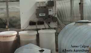
Figure 18. Typical fertilizer feed system with two fertilizer stock tanks and computerized control of pH and E.C.
Feed monitoring stations are established throughout the crop, one or two stations per every 0.4 hectare (1 acre) of greenhouse area are usually sufficient, but having one monitoring station for every watering "zone" of the greenhouse is a good idea. The purpose of the monitoring station is to measure the volume of feed delivered to the individual plants, and to determine the volume of feed solution leachate, or "over-drain" that is flowing past the plants and out of the root zone over the course of the day. The E.C. and pH of the feed solution is taken on a daily basis, as is the E.C. and pH of the leachate.
Daily monitoring the percentage of feed solution volume flowing through the root zone environment, the sawdust bags, or rockwool slabs etc., is used to adjust the volume of feed solution delivered to the plants. The E.C. of the leachate is used to make adjustments on the feed solution E.C. Monitoring the pH of the feed and leachate helps to ensure that the correct pH is being fed to the crop and gives an indication of what is happening in the root zone with respect to pH. Optimum feed pH is approximately 5.8, and this pH optimum also applies to the root environment as well. Generally the activity of the roots tends to raise the pH in the root environment and feeding at a lower pH can help counteract this rise in pH.
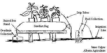
Figure 19. General schematic of a fertilizer feed monitoring station.
It is not recommended to feed at a pH of lower than 5.5 when attempting to lower the pH in the root zone. In addition to feeding at a pH of 5.5, the use of ammonium nitrate at 2 to 5 ppm of ammonium nitrogen (NH4 - N) will help to lower the pH of the root zone due to the acidifying effect of this fertilizer.
A schematic of a typical feed monitoring station is presented in figure 19. In addition to monitoring the feed and leachate, recording the leachate percentage, feed and leachate E.C. and pH can be used as a tool to chart the performance of the crop with respect to these recorded values over time, and in relationship to other parameters including the amount and intensity of available light.
The amount of nutrient solution delivered to the plant on a daily basis can be determined by the percentage over-drain or leachate that is recovered from the plants over the course of the day. Leaching, or allowing a certain percentage of nutrient solution applied to the crop, to pass through the root system, allows for a flushing of the root zone to avoid the accumulation of salts. Generally, when the plants are young, a percentage leachate of 5 to 10% is a good target. As the plants develop, the amount of water required to attain this over-drain target increases. As the season progresses and the light levels increase and the plants mature and begin to bear fruit, the over-drain targets increase to 20 to 30%. Generally these higher over-drain targets apply as the high light period of the year begins, usually in June. As the percentage over-drain decreases, the leachate E.C. increases, that is, the amount of salts in the root zone increases. The general rule for managing the level of salts in the root zone is that the root zone E.C. should not be greater than 1.0 mmho above the feed E.C.
The design of the feed solution is based on delivering adequate nutrition to the plants, and these feed programs usually have an E.C. 2.5 mmhos (this is largely dependent on the E.C. of the irrigation water). With the optimum feed solution E.C. at approximately 2.5 - 3.0 mmhos, the salt levels in the root zone should be maintained at around 3.5 - 4.0 mmhos. Early in the crop cycle, the salt levels in the root zone can be maintained at the proper target fairly easily by increasing the volume of nutrient solution delivered to the plant to ensure a 5 to 10% over-drain. As the season progresses and the water has been increased so that the upper limit of 30% over-drain has been reached, and the E.C. of the over-drain continues to climb above the target of 3.5 - 4.0 mmhos, the E.C. of the solution can be dropped. The reduction in feed solution E.C. is accomplished in stages with gradual, incremental reductions in feed E.C. in the order of 0.2 mmhos every 2 to 3 days. It is never advised to apply straight water to the plants in order to lower the root zone E.C., since the rapid reduction in root zone E.C. and increased pH can reduce the performance of the crop and compromise the health of the roots (Maree 1994).
During periods when the plants are in a rapid stage of growth, the E.C. in the root zone can be below that of the feed solution. For example, the feed can be at 2.5 mmhos while the leachate E.C. may be a 2.0 mmhos. This is an indicator that the plants require more nutrients and the feed E.C. should be increased in increments in the order of 0.2 mmhos until the E.C. in the root zone begins to approach the upper target limit of 4.0 mmhos.
By varying the volume and E.C. of nutrient solution delivered to the plants, in accordance to the leachate over-drain and E.C. targets, it is possible to optimize the delivery of adequate water and nutrients to the crop without over watering and over fertilizing. Applying too much or too little water can compromise the health and performance of the crop.
The delivery of water to the plants occurs over the course of the entire day. Watering can be scheduled by using a time clock or in more sophisticated systems the watering events can be triggered by the amount of incoming light received by the greenhouse. In general, the greater the ability to control the delivery of water, the greater the ability to maximize crop performance.
A starting point for watering the crop early in the crop cycle would be to apply water every half hour from one half hour after sunrise to approximately one hour before sunset. The amount of water required to meet the over-drain target is divided amongst the waterings based on the duration of the individual waterings. For example if a 40 second watering delivers 100 ml of water, then 10 watering events are required to deliver one litre of water. When more than a litre of water is required in one day the duration of the individual watering events can be increased, or the number of watering events can be increased or both. Generally, as the crop matures, it is better to increase the frequency of watering events than the duration of each event. If the watering system allows the variation of the frequency and duration of the watering events over the course of the day, then it is possible to increase the frequency and/or duration of the watering events during the high light period of the day without necessarily increasing the duration of the early morning or late afternoon watering events.
Watering frequency can be used to help direct the vegetative/generative balance of the plant. For any given volume of water that is delivered to the plants, the more frequent the waterings throughout the day, the more the plant will be directed to grow vegetatively. The longer the duration between waterings, the stronger the generative signal sent to the plant. Frequent watering during the summer months in Alberta can help balance plants that are overly generative due to the intense sunlight, high temperatures and low relative humidity.
When the concept of percent over-drain is discussed, it is preferable to obtain the majority of the over-drain during the high light period of the day. The first of the over-drain should start to occur at 10:00 am and the greater part of the daily over-drain target should be reached by 2:00 to 3:00 p.m. Having the capability of varying the duration of the watering events over the course of the day allows for more nutrient feed being delivered to the plants between 10:00 am and 2:00 - 3:00 p.m.
The use of over-drain targets is one way to ensure the plants are receiving adequate water throughout the day. Another strong indicator of whether or not the plants have received adequate water during the previous day is whether the growing points, or the tops of the plants have a light green color early in the morning. Over the course of the day when the plant is under transpiration stress, the color of the plants will progress from a light green to a darker blue-green. If the plants have received adequate water throughout the previous day, the light green color will return overnight as the plant recovers and improves its water status. If the plants remain a darker bluish-green in the early morning, the amount of water delivered the previous day was inadequate. Usually, this means that the over-drain target for the previous day have not been met and the amount of nutrient solution delivered to the plants has to be increased.
During the summer months, under continuous periods of intense light, the plants may not have recovered their water status overnight even when the daily over-drain targets have been met. The plants begin the day a dark blue-green in color, an indication that they are already under water stress, even though the day has just begun. Under these circumstances the overdrain targets for the day could be increased, but there is the associated risk of over-watering and decreasing root health and performance. In these cases it is advisable to consider one or two night waterings, one at approximately 10:00 p.m. or one at 2:00 am or both. Usually the night watering events are the same length of time as the minimum watering duration applied during the day. Night watering can also help increase the rate of fruit development, but there is an associated risk of fruit splitting if too much water is applied at night. The night waterings should not be continued indefinitely and the decision to use night watering events and to continue with night watering has to be based on the assessed needs of the crop.
The management of the feed solution, and its delivery to the crop has to be relatively flexible to meet the changing needs of the crop. With experience, growers gain more confidence and skill in meeting and anticipating the changing needs of the crop throughout the crop cycle and through periods of fluctuating light levels. The general information presented in this section serves as a starting point and by following the principles of over-drain management, E.C. and pH monitoring and correction, a successful strategy for delivery of water and nutrients can be established.
As with many things there is no one "right" way to apply water and nutrients to the crop. The use of leaching, although ensuring that salt levels do not accumulate to high levels in the root zone, does result in some "waste" of fertilizer solution as runoff. There are strategies that can be employed to minimize the waste associated with leaching. Collection and recirculation of the leachate, with an associated partial sterilization, or biofiltration of the nutrient solution is one approach (Portree 1996, Ng and van der Gulik 1999). The sterilization or biofiltration steps are required in order to minimize the disease risk associated with recycling nutrient solutions. Some estimates place the fertilizer cost savings at between 30 to 40% when recirculation is used (Portree 1996). In addition to being economical, recycling nutrient solutions is an environmentally sound practice (Zekki et al 1996).
There is a limit to how long nutrient solutions can be recirculated, prolonged recycling of the same solution can negatively affect growth and yield. This is primarily associated with the accumulation of sulfate ions in the solution (Zekki et al 1996). In addition to sulfates, chlorides and bicarbonates also have a tendency to accumulate and can influence crop growth (Zekki et al 1996). The progressive accumulation of sulfates in recirculating solutions require occasional "refreshing" of the solution whereby the solution would have to be allowed to leave the greenhouse as waste (Zekki et al 1996). |
|